B2 III: RNAseq - bcfgothenburg/HT23 GitHub Wiki
The purpose of these exercises is to introduce you to the post-processing of RNA-seq data. You will start by assessing the quality of the sequencing data. Then you will perform a standard differential expression analysis as well as a pathway analysis.
Your task is to identify possible differentially expressed (DE) genes that are specific to individuals infected with visceral leishmaniasis (VL).

Due to limit in time, you won't be running some analysis, but rather interpreting the results. These analyses can be performed using a web server (Galaxy, for instance), where you can choose an array of tools to produce the same output files you will be provided with. Throughout the practical, we include the command lines we have used in a linux environment to generate the output files.
Leishmaniasis, is a disease caused by protozoan parasites of the genus Leishmania and spread by the bite of certain types of sandflies. Manuela S. L. Nascimento and others (2016) investigated signature genes in human during this infection using RNAseq. The raw data (fastq files) were downloaded from ENA (European Nucleotide Archive) under the project E-MTAB-4902.
These are the samples used:
| Run Accession | Type | ID |
|---|---|---|
| ERR1523942 | Normal | Ctrl1 |
| ERR1523943 | Normal | Ctrl2 |
| ERR1523944 | Normal | Ctrl3 |
| ERR1523945 | Normal | Ctrl4 |
| ERR1523946 | Normal | Ctrl5 |
| ERR1523947 | Visceral Leishmaniasis | VL1 |
| ERR1523948 | Visceral Leishmaniasis | VL2 |
| ERR1523949 | Visceral Leishmaniasis | VL3 |
- Download the files from the
RNAseqfolder, as indicated in the course web platform
We will start by looking at the quality of the sequencing data. FastQC is a program that generates general statistics of sequencing data. Since we have a lot of samples, it is convenient to merge all the reports and stats files. We can achieve this by using MultiQC:
# running fastqc for all the samples
fastqc -o . *fastq.gz

# Running multiqc to gather all html reports
multiqc --filename multiqc_report_Raw_data \ # output filename
    --title Raw_data                       \ # title in the html file
. # output directory- Open
multiqc_report_Raw_data.htmlin your web browser.
Q1. What are your conclusions about the quality of the sequencing?
There are a lot of tools that can help us to trim our data based on quality, either by removing the low quality ends,
possible adapters left, etc. Trim Galore!
offers both quality and adapter trimming as well as quality control. As we can run fastqc on the go, the next step is to gather all the reports with multiqc:
# processing R1 and R2 simultaneously
trim_galore --paired       \ # processes the data as paired-end files (both reads must pass the filters to be retained)
    --quality 20           \ # trims low-quality ends from the reads in addition to adapter removal
    --max_n 0.2            \ # discards reads that exceed the number of N's in the read
    --length 40            \ # discards reads that became shorter than the set length
    --fastqc               \ # runs FastQC on the trimmed set
    -o trim_galore         \ # sets the output directory
    Ctrl1_1.fastq.gz       \ # Read 1 file
    Ctrl1_2.fastq.gz         # Read 2 file

# running multiqc to gather all html reports
multiqc --filename multiqc_report_Trimmed_data --title Trimmed_data . - Open the report file from the trimmed data
multiqc_report_Trimmed_data.html.
Q2. How many reads were trimmed? If you didn't use the Universal Illumina adapter, how would you specify your adapter in the command line above? Hint: Look in the manual page for TrimGalore!
Now that we have a good quality dataset, we need to align the reads to the reference genome. There are several short read aligners that can handle the non-contiguous transcript structure of RNAseq experiments. Here we will be using STAR. The basic workflow includes 2 steps: 1) Generating the genome indexes (which is done only once) and 2) Mapping the reads to the genome.
# generating genome indexes with basic options
STAR --runMode genomeGenerate                              \ # to run the genome indices generation job
    --genomeDir /db/STARIndex/2.7.4a                       \ # directory where the genome is stored
    --genomeFastaFiles /db/Homo_sapiens/Ensembl/GRCh37     \ # genome reference sequence
    --sjdbGTFfile db/Homo_sapiens/Ensembl/GRCh37/genes.gtf \ # transcript annotation in GTF format
    --runThreadN 10                                        \ # number of threads to be used

# mapping trimmed reads with default parameters for one sample
STAR --genomeDir /db/STARIndex/2.7.4a                       \ # directory where the indexes are stored
    --readFilesIn  Ctrl1_1_val_1.fq Ctrl1_2_val_2.fq        \ # input fastq files
    --readFilesCommand gunzip -c                            \ # to uncompress the fastq files
    --outFileNamePrefix Ctrl1/Ctrl1                         \ # output directory
    --sjdbGTFfile /db/Homo_sapiens/Ensembl/GRCh37/genes.gtf \ # transcript annotation in GTF format
    --runThreadN 10                                         \ # number of threads to be used
    --outSAMtype BAM SortedByCoordinate                       # output alignment format
Creating statistics of the alignments will help us to assess the data. We can use samtools, a suite of programs
for interacting with high-throughput sequencing data, to generate overall statistics and then use RSeQC, a program consisting of multiple python scripts, to evaluate in more detail some aspects of the data. Then we can then gather the info with MultiQC:
# calculating simple statistics
samtools flagstat Ctrl1Aligned.sortedByCoord.out.bam > Ctrl1Aligned.sortedByCoord.out.bam.flagstat
samtools idxstats Ctrl1Aligned.sortedByCoord.out.bam > Ctrl1Aligned.sortedByCoord.out.bam.idxstats

# calculating how mapped reads were distributed over genome feature
read_distribution.py --input-file Ctrl1Aligned.sortedByCoord.out.bam \ # alignment file
    --refgene /db/Homo_sapiens/Ensembl/GRCh37/gene.bed               \ # Reference gene model in bed format
    > Ctrl1Aligned.sortedByCoord.out.bam.distribution                  # output file name

# inferring which protocol was used: unstranded, stranded or reverse stranded
infer_experiment.py --input-file Ctrl1Aligned.sortedByCoord.out.bam \ # alignment file
    --refgene /db/Homo_sapiens/Ensembl/GRCh37/gene.bed              \ # Reference gene model in bed format
    > $i.infer_experiment                                             # output file name

# calculating the coverage over the gene body
geneBody_coverage.py
    --input Ctrl1Aligned.sortedByCoord.out.bam, Ctrl2Aligned.sortedByCoord.out.bam, ..., \ # all alignment files to analyze
    --refgene /db/Homo_sapiens/Ensembl/GRCh37/gene.bed                                   \ # Reference gene model in bed format
    --out-prefix rnaseq                                                                  \ # output file name
    --format png                                                                           # output format

# running multiqc to gather all html reports
multiqc --filename multiqc_report_Aligned_data --title Aligned_data .- Open
multiqc_report_Aligned_data.htmlandrnaseq.geneBodyCoverage.curves.pngin your web browser.
Q3. Have all the reads been mapped to the reference genome? Which feature has the most reads, does that correlate with the type of sequencing we have? Is it a stranded library? Do you think we have a problem with fragmentation?
Remember that a tiled data file file (.tdf) is a binary file that contains data that has been pre-processed for faster display in IGV.
We generated the tdf files for all the samples with this command:
# generating tdf files
igvtools count                                                           \ # tool used
     Ctrl1Aligned.sortedByCoord.out.bam                                  \ # input filename
     Ctrl1Aligned.sortedByCoord.out.tdf                                  \ # output filename
/db/Homo_sapiens/Ensembl/GRCh37/Sequence/WholeGenomeFasta/genome.fa \ # path to the genome file- Select one Ctrl and one VL sample and load their corresponding
BAMandtdffiles inIGV - Right-click in the
Annotation trackto see all known/annotated splice forms - Try the
view-as-pairsoption
Q4. Are the benefits using a “splice-junction-aware” aligner such as STAR visible? How many transcript isoforms are known (in RefSeq) for the BRCA1 gene? Do all of them seem to be expressed in this sample?
- Color the alignment by
First of pair strand
Q5. Is this dataset “stranded” or “unstranded”?
- Right-click in the
tdf track - Select
Set Data Range - Set
Maxto 10000
Q6. Are there any genes with exceptional expression level? Which ones? Are they annotated? What kind of genes are they?
- Zoom in one of these genes
- In the tool bar
- Click the
Define a Region of Interesticon
- Click the
- In the data panel
- Click at the start of the gene and then at the end of the gene
You will see a red line -
Right-clickon the red line - Select
Copy sequence(now you have the sequence in the clipboard)
- Click at the start of the gene and then at the end of the gene
- Try to annotate the sequence by using for instance BLAST
Q7. Could you annotate the sequence? what is it?
Counting reads that map to a gene may sound trivial. HTseq-count, a python package that help us to process data from high-throughput sequencing assays, has a nice figure illustrating different cases.
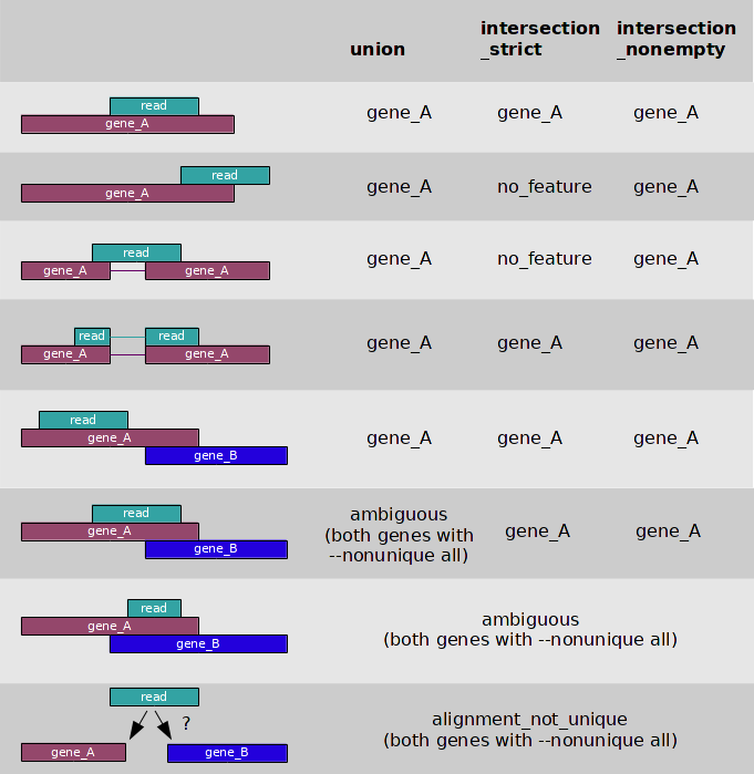
Q8. Would you prefer any of the 3 modes (union, intersection_strict, intersection_nonempty) as counting strategy? Why?
featureCounts is a program for counting reads to genomic features such as genes, exons, promoters and genomic bins. It is quicker than other tools and it can generate a matrix on the go, which would be the input to the Differential expression analysis:
featureCounts -p                                                              \ # indicative that we are using paired-end data
    --countReadPairs                                                          \ # Count fragments instead of reads
    -s 2                                                                      \ # library strandness: reverse
    -t exon                                                                   \ # feature to count
    -a /db/Homo_sapiens/Ensembl/GRCh37/genes.gtf                              \ # transcript annotation
    -o VL.counts                                                              \ # output file name
    Ctrl1Aligned.sortedByCoord.out.bam Ctrl2Aligned.sortedByCoord.out.bam ... \ # alignment files
Q9. Why are we using
reverseas strand-specific assay?
- Have a look at the
VL.countsfile, you can directly open in excel
Q10. Can you identify any DE gene? Is it possible to make any comparison among the samples?
The output format of featurecounts is a tab separated file, first two rows are the command and the header. First column is geneid, columns 2-6 contain additional information. The count information is starting from column 7.
'# Program:featureCounts v2.0.6; Command:"featureCounts" "-p" "--countReadPairs" "-s" "2" "-t" "exon" "-a" "/home/db/Homo_sapiens/Ensembl/GRCh37/Annotation/Genes/genes.gtf" "-o" "VL.counts" "Ctrl1Aligned.sortedByCoord.out.bam" "Ctrl2Aligned.sortedByCoord.out.bam" "Ctrl3Aligned.sortedByCoord.out.bam" "Ctrl4Aligned.sortedByCoord.out.bam" "Ctrl5Aligned.sortedByCoord.out.bam" "VL1Aligned.sortedByCoord.out.bam" "VL2Aligned.sortedByCoord.out.bam" "VL3Aligned.sortedByCoord.out.bam"
Geneid  Chr     Start   End     Strand  Length  Ctrl1Aligned.sortedByCoord.out.bam      Ctrl2Aligned.sortedByCoord.out.bam      Ctrl3Aligned.sortedByCoord.out.bam      Ctrl4Aligned.sortedByCoord.out.bam       Ctrl5Aligned.sortedByCoord.out.bam      VL1Aligned.sortedByCoord.out.bam        VL2Aligned.sortedByCoord.out.bam        VL3Aligned.sortedByCoord.out.bam
ENSG00000223972 1;1;1;1;1;1;1;1;1;1;1;1;1;1;1;1 11869;11872;11874;12010;12179;12595;12613;12613;12613;12975;13221;13221;13225;13403;13453;13661 12227;12227;12227;12057;12227;12721;12697;12721;12721;13052;13374;14409;14412;13655;13670;14409  +;+;+;+;+;+;+;+;+;+;+;+;+;+;+;+ 1756    0       16      17      20      9       1       0       0
When reading in the count matrix into R later we will have in mind that we want to skip the first row containing the command, and we only keep the first column and the count columns.
There are different methods to quantify genes, and there has been a lot of debate as to which is the best one. Here you can find an attempt to clarify some terms.
Q11. In your opinion, which is the best counting method? RPKM, FKPM, TPM? Why?
There are many software packages for differential expression analysis of RNA-seq data. Several tools, such as DESeq2 and edgeR, start from read counts per gene and use the discrete nature of the data to do statistical tests appropriate for this kind of data.
Here you will use DESeq2, an R package that estimates variance-mean dependence in count data from high-throughput sequencing assays and tests for differential expression based on a model using the negative binomial distribution.
Start R in your local computer.
Select your working directory (where you have the VL.counts file) by clicking: Session -> Set Working Directory -> Choose directory
Most of the code is copy/paste. Modify when asked, this will be indicated in CAPITAL letters
Install these libraries (if you already have them, go ahead and load them):
if (!require("BiocManager", quietly = TRUE))
    install.packages("BiocManager")

BiocManager::install("DESeq2")
BiocManager::install("AnnotationDbi")
BiocManager::install("org.Hs.eg.db")
install.packages('pheatmap')
Load the libraries:
library(DESeq2)
library(pheatmap)
library(AnnotationDbi)
library(org.Hs.eg.db)
Now, load the gene counts:
# Reading the sample information
counts <- read.table("VL.counts",
                     header    = TRUE,
                     row.names = 1,
                     sep       = "\t",
                     as.is     = TRUE)
head(counts)

# Displaying the dimensions of the data
dim(counts)

# Extract the count columns
counts<-counts[,6:ncol(counts)] # Count columns start from column 6 (as first columns is now the rowname)


# Remove name Aligned.sortedByCoord.out.bam string from the sample names
colnames(counts)<-gsub(pattern="Aligned.sortedByCoord.out.bam",replacement="",colnames(counts))

# look at the first rows
head(counts)
Let's define the metadata for our samples. This will set the colors to be displayed in our graphs and define the grouping for the analysis:
# Defining the sample names
sampleNames <- colnames(counts)
sampleNames

# Defining the sample grouping
conditionNames <- data.frame(condition = c(rep("ADD_A_NAME_FOR_THE_CONTROLS",5), rep("ADD_A_NAME_FOR_THE_VL_SAMPLES",3)))
conditionNames

# Defining the Control and the Visceral Leishmaniasis group for plotting
annotation_col <- data.frame(
  Type = c(rep("ADD_THE_SAME_NAME_FOR_THE_CONTROLS",5), rep("ADD_THE_SAME_NAME_FOR_THE_VL_SAMPLES",3))
)
annotation_col

# Defining the colors by group for plotting
annotation_colors <- list(
  Type = c(ADD_THE_SAME_NAME_FOR_THE_CONTROLS="ADD_A_COLOR_NAME", ADD_THE_SAME_NAME_FOR_THE_VL_SAMPLES="ADD_A_COLOR_NAME")
)
annotation_colors

rownames(annotation_col) = sampleNames
Now we need to construct the main data object. The DESeqDataSetFromMatrix function constructs a DESeq2 data set object. This integrates the counts, the samples description and the experimental design:
# Creating the DESeqDataSet
dds <- DESeqDataSetFromMatrix(countData = counts,
                              colData   = conditionNames,
                              design    =~ condition)
dds
One of the first things that we need to do is to assess the overall similarity between the samples. We can create a PCA plot:
# Data transformation
rld <- rlogTransformation(dds)

# Ploting PCA
plotPCA(rld)
Or we can look at the Euclidean distance:
# Calculating distance among samples
sampleDist <- dist(t(assay(rld)))
sampleDistMtx <- as.matrix(sampleDist)

# Plotting the distances
pheatmap(sampleDistMtx,
         cluster_rows      = hclust(sampleDist),
         cluster_cols      = hclust(sampleDist),
         main              = "ADD_A_TITLE",
         fontsize_row      = 12,
         annotation_col    = annotation_col,
         annotation_colors = annotation_colors)
Q12. Is the clustering consistent with our different groups?
Now we can proceed with the differential expression testing. The DESeq function does all the hard work, it basically performs three steps:
- Compute a scaling factor for each sample to account for differences in read depth and complexity between samples
- Estimate the variance among samples
- Test for differences in expression among groups
# DE test
dds <- DESeq(dds)
head(dds)

# Extracting the results
res <- results(dds)
head(res)
Q13. How many genes do you have in the result matrix? use
nrow(res)
Remember that since we are doing a lot of tests, as many as genes in our experiment, we need to correct our pvalues. DESeq already did this while testing for differences among our groups, so let's create a histogram of these adjusted pvalues and an MA-plot to inspect if there is any enrichment of DE genes:
# Padjusted histogram

breaks      = ADD_A_NUMBER
color       = ADD_A_COLOR
borderColor = ADD_A_BODER_COLOR

hist(res$padj,
     breaks = breaks,
     col    = color,
     border = borderColor,
     main   = "ADD_A_TITLE",
     xlab   = "ADD_X_LABEL")

# log2FoldChange histogram

hist(res$log2FoldChange,
     breaks = breaks,
     col    = color,
     border = borderColor,
     main   = "ADD_A_TITLE",
     xlab   = "ADD_X_LABEL")

# MA-plot

foldChange_yLimit=ADD_FOLDCHANGE_VALUE_BASED_ON_THE_PREVIOUS_GRAPH

plotMA(res,
       main = "ADD_TITLE",
       ylim = c(-foldChange_yLimit, foldChange_yLimit))
Q14. What does the histogram tell you? What are the highest and lowest fold changes (approx) found in our dataset?
There are genes that have very low counts across all the samples, these can't be tested for DE so they end up with an NA p-adj. Let's remove them:
# checking how many genes have
nrow(res)

# checking how many genes have NA
sum(is.na(res$padj))

# removing the NA padj
res <- res[ ! is.na(res$padj), ]

# checking how many genes have
nrow(res)
Q15. How many genes were removed?
We can now explore our data a little bit more. We can focus on genes that are significant according to some criteria: false discovery rate (FDR) or log fold change. For example, we can filter the results so that 1% are expected to be false positives (genes with no actual difference in expression):
#  selecting statistically significant genes
padjusted = ADD_PADJ_THRESHOLD

res_sig <- res[ which(res$padj < padjusted), ]
res_sig
Q16. How many significant genes do you have?
To see the top 20 most upregulated genes:
# selecting top genes to show
top = ADD_NUMBER_OF_GENES_TO_SHOW

print(as.matrix(res_sig[ order(res_sig$log2FoldChange, decreasing=TRUE),][1:top,]))
Q17. Make a note of the genes.
Q18. Change the
decreasingargument toFALSE, what type of genes do you get? Make also a note of these genes.
It is also important to have a graphical representation of these results. A heatmap of the significantly DE genes can be generated as follows:
# Selecting the rlog-transformed counts of the DE genes
sig2heatmap <- assay(rld)[rownames(assay(rld))%in%rownames(res_sig),]

# Calculating the difference of the counts to the mean value
sig2heatmap_Mean <- sig2heatmap - rowMeans(sig2heatmap)

# Plotting
pheatmap(sig2heatmap_Mean,
         main              = "ADD_TITLE",
         annotation_col    = annotation_col,
         annotation_colors = annotation_colors,
         show_rownames     = FALSE)
Q19. What does the heatmap tell you?
You can of course plot the top 20 most significant genes:
# Selecting the top 20 genes based on adjusted pvalue
res_top <- res_sig[order(res_sig$padj),][1:top,]

# Selecting the rlog-transformed counts of the DE genes
top2heatmap <- assay(rld)[rownames(assay(rld))%in%rownames(res_top),]

# Calculating the difference of the counts to the mean value
top2heatmap_Mean <- top2heatmap - rowMeans(top2heatmap)

# Plotting
pheatmap(top2heatmap_Mean,
         main              = "ADD_TITLE",
         annotation_col    = annotation_col,
         annotation_colors = annotation_colors)
Q20. What can you conclude from this heatmap? Are the plotted genes in your top 20 most up/down regulated list?
It is also possible to plot the counts for individual genes:
plotCounts(dds, gene="ENSG00000178752", intgroup="condition")Q21. Plot a gene with high pvalue, is there an evident difference between Ctrl and VL?
Adding different types of identifiers to our significant genes help us to use web-based tools, especially when they require a specific identifier (different to the ones we have for instance). Let's use R this time!
# mapping ensembl identifier to gene symbols
res$symbol<-mapIds(org.Hs.eg.db,
                   keys    = row.names(res),
                   column  = "SYMBOL",
                   keytype = "ENSEMBL")
res_ann<-res
head(res_ann)
Now you can save these results as this file can be used in downstream analyses. However we will not use it as we have the results in the same R session:
# saving results as a tab delimited file
write.table(res_ann,
            file      = "VL_vs_Ctrl_DE.txt",
            col.names = TRUE,
            row.names = TRUE,
            sep       = "\t",
            quote     = FALSE,
            na        = "NA")
You can of course create tables for publishing. For example, you can choose the columns you need and format them. For this example we are using the kableExtra package. Install it and load it if you do not have it:
# installing and loading the library
install.packages("kableExtra")
library("kableExtra")

# generating a table
knitr::kable(head(res[c(2,5,6,7)]), caption="Top 10 DE genes in Leishmaniasis")The resulting gene list from the DE analysis can be very long and hard to interpret. In order to summarize the genes one could perform a Gene Ontology analysis (GO). Gene ontologies describes 3 different aspects:
- Molecular function - A molecular process that can be carried out by the action of a single macromolecular machine, usually via direct physical interactions with other molecular entities
- Cellular component - A location, relative to cellular compartments and structures, occupied by a macromolecular machine when it carries out a molecular function
- Biological process - A biological process represents a specific objective that the organism is genetically programmed to achieve
You can read more about Gene Ontologies here
In this part of the practical we will use our significant gene list from the differential expression analysis to perform a gene set enrichment analysis to find affected GO terms.
First let's install the tool. If you already have them, just load them:
# installing libraries
BiocManager::install("topGO")
BiocManager::install("Rgraphviz")

# loading libraries
library(topGO)
library(Rgraphviz)
We start by generating the topgo object looking at the ontology biological process (BP).
# Defining the ontology to use: BP, MF, CC
ONT = "BP"

# Creating the dataset with padj<0.01
res_GO <- new("topGOdata",
              description = "Leishmaniasis project",
              ontology    = ONT,
              allGenes    = setNames(res$padj, rownames(res)),
              geneSel     = function(x) x<0.01,
              nodeSize    = 10,
              mapping     = "org.Hs.eg.db",
              ID          = "ensembl",
              annot       = annFUN.org)

# Displaying the info
res_GO
Q22. Looking at the object how many significant genes are used in the analysis, why are not all 1230 significant genes used?
Then we perform the enrichment test. There are several tests, and here we will use Kolmogorv Smirnov. This test is used when you have manipulated data as input (P-values). KS test compares the distribution of P-values expected at random to the observed distribution of P-values. There are different methods to use in topGO, here we use the default one, weigth01, which is a mixture of the methods elim (a method that goes through the hierarchy of the go terms and discards significant descendant GO-terms if it hits further up) and weight (a method that compares the significant scores to detect the most significant term in the hierarchy):
# Running the statistical test
resultKS <- runTest(res_GO,
                    algorithm = "weight01",
                    statistic = "ks") # Statistical test KS

# Creating a table with the results
res_GO_table_BP <- GenTable(res_GO,
                            Weigth1_KS = resultKS,
                            orderBy    = "Weigth1_KS",
                            ranksOf    = "Weigth1_KS",
                            topNodes   = 15)  #top 15 GO to a table
# Displaying the results
res_GO_table_BP
You read the different columns as described below:
- GO.ID - Gene ontology ID
- Term - Describing the go term
- Annotated - How many genes does the GO term contain
- Significant - How many of these GO terms are significantly enriched in your list
- Expected - How many would you expect by chance
- Weigth1_KS - P-value from the KS test with the weight method
The majority of the processes affected seem to be linked to the mitochondria.
You can also visualize the results in the console.
# displaying the GO graphic
showSigOfNodes(res_GO,
               score(resultKS),
               firstSigNode = 1,
               useInfo      = 'all')
Or save the plot directly to a pdf
# printing the graph into a file,
# saved in the location you set as working directory
printGraph(res_GO,
           resultKS,
           firstSigNodes = 1,
           fn.prefix     = "tGO",
           useInfo       = "all",
           pdfSW         = TRUE)
In this graph you can see the significant GO-Term GO:0015670 carbon dioxide transport in the red square at the lower part of the plot and its location in the hierarchy.
Repeat the same analysis focusing on the cellular component (CC). Hint: you just need to replace ONT="BP" to ONT="CC" and when running the GeneTable() function, save it as res_GO_table_CC
Q23. Which is the most significant
cellular componentwe find? How significant is it based on the KS test?
Now, do the same analysis with the final GO class molecular function (MF). Hint: you just need to set ONT="MF" and when running the GeneTable() function, save it as res_GO_table_MF
Q24. Which is the most significant
molecular functionwe find? How significant is it based on the KS test?
Let's merge the top 15 GO terms from each class and view it in a table:
# Merging results into one table
Results_Topgo <- cbind(BP=res_GO_table_BP$Term,
                       CC=res_GO_table_CC$Term,
                       MF=res_GO_table_MF$Term)

# Visualizing the table
knitr::kable(Results_Topgo, caption = "Top 15 significant GOs")
Q25. Do you find any hits in the different go terms that are known to be linked to visceral leishmaniasis?
Home: Bioinformatics 2
Developed by Sanna Abrahamsson, 2021. Modified by Sanna Abrahamsson and Marcela Dávila, 2023.