Lecture 6 - bancron/stanford-cs224n GitHub Wiki

Lecture video: link

RNN Language Models

Last lecture we learned about language models, n-gram language models, and recurrent neural networks (RNNs).

Recall that we take a sequence of words, convert them to word embeddings, and then run the recurrent layer where at each point we have a previous hidden state, then feed the previous hidden state and the encoding of the word into the next hidden state. Based on that we compute a new hidden state to pass into the next word in the sequence. At each time step, we also generate an output by feeding the hidden layer into a softmax layer, which gives us a probability distribution over words.

Training

How do we train this? We take a large corpus of text (long sequence of words). We feed it into the RNN-LM: take prefixes of that sequence, and based on the prefix, calculate the probability distribution of the word that comes next. Then we train the model using the loss function cross-entropy loss, the the negative log likelihood, between the predicted word and the true next word. Then we average this over all time steps to get the overall loss for the entire training set.

This is known as "teacher forcing". We will start with a prefix (e.g. "the students"), then predict one time step forward. After that we set the prefix to e.g. "the students opened": resetting the state to what actually happened in the corpus (ignoring, for example, if the model did not predict "opened").

Computing the loss and gradients across the entire corpus at each step is too expensive. In practice, we cut it into smaller pieces such as sentences or documents, compute gradients from those, update the weights, and repeat. We also typically use a batch of sentences such as 32 sentences of a similar length rather than just a single one.

Backpropagation for RNNs

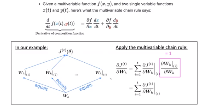
What is the derivative of Jt(θ) w.r.t. the repeated weight matrix Wh? We look at it in each position and calculate the partials of Jt with respect to Wh in position t=1, t=2 etc, and sum up all of those partials.

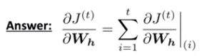
The gradient w.r.t. a repeated weight is the sum of the gradient w.r.t. each time it appears. Note that this doesn't mean that it is t times ∂Jt/∂Wh, because Wh is used repeatedly through the sequence, and each time a new upstream gradient is fed into it, so each value in the sum is completely different.

If we have a multivariable function f(x, y) and two single variable functions x(t) and y(t), the multivariable chain rule ("gradients sum at outward branches") says:

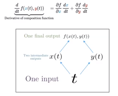
The final output is f(x(t), y(t)).

We can generalize this to many pieces. We have one Wh matrix, and we use this to update the hidden state across time 1 ... time t. This has many outward branches, and we will sum the gradient path at each one. But the gradient path just uses Wh at each position, so (∂Wh at time i) / ∂Wh is just equal to 1.

We work out derivatives w.r.t. the hidden layer, then w.r.t. Wh at the last time step (one update for Wh), then the t-1 time step (another update for Wh) which we sum onto Wh. We continue this all the way to the beginning to create a total update for Wh. This is called "backpropagation through time".

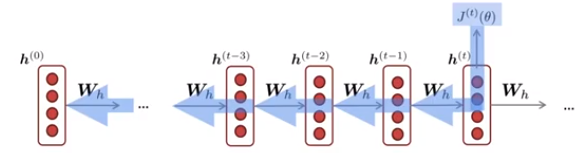
We want to accumulate all the updates and then apply them all once at the end rather than changing the Wh matrix as we go; the latter would be invalid because the forward calculations were done with the constant Wh from the preceding state.

If we are doing this for sentences we can go back to the beginning of the sentence. If the data is much longer than a sentence, we may do truncated backpropagation, which chooses some constant (e.g. 20) and only updates the Wh matrix back that many steps.

Other uses of RNNs

Text generation

As with an n-gram language model, we can generate text by repeated sampling. We start with an initial state (normally a zero vector) and an initial input, e.g. the first word or nothing (to generate entire sentences from scratch). If we want to do the latter, we use a beginning-of-sequence token for the initial input. At each time step we sample to choose some word, then take that word and use it at the input at the next time step. We end by using an end-of-sequence symbol and waiting until that symbol is generated. This will generate text in different styles based on the data that the LM was trained on.

As compared to an n-gram LM, training the RNN will be much slower, but text generation from the model will be much faster.

Evaluating LMs

The standard evaluation metric for language models is perplexity. We take text (which was not in the training data), condition on the first t words and calculate the probability of the actual next word, repeating at each position. Then take the inverse of that probability and raise it to 1/T (where T is the total number of words). This is the geometric mean of the inverse probabilities.

A simpler way to look at this is that the perplexity is simply the cross-entropy loss J(θ), exponentiated. Note that lower perplexity is better. If the perplexity is N, this is equivalent to the uncertainty of tossing an N-sided die and having it come up 1.

Traditional n-gram language models have a perplexity of over 100; very good ones can get as low as 67. Increasingly complex RNNs can get a perplexity in the 60s, LSTMs (long short term memory, to be covered in a moment) can get the perplexity as low as 30. Some words are extremely determined, e.g. "he gave her a napkin and she said thank" -> "you", but some are very underdetermined, e.g. "he looked out the window and saw a" -> ??. No LM in the world could get that right consistently.

Why should we care about language modeling?

• Language modeling is a benchmark task to help us measure our progress on understanding language, both the structure of language and the structure of the real world.
• Language modeling is a subcomponent of many NLP tasks, especially those involving generating text or estimating the probability of text.
  • Predictive typing
  • Speech recognition
  • Handwriting recognition
  • Spelling and grammar correction
  • ...

Recall that:

• A language model is a system that predicts the next word.

• An RNN is a family of neural networks that:

  • take sequential input of any length
  • apply the same weights on each step
  • and can optionally produce output on each step.

These are not equivalent. RNNs are a great way to build an LM, but they are also useful for many other tasks.

Sequence tagging: take a sequence of words and tag them with parts of speech (determiner, adjective, noun, etc.).

Sentiment classification: classify a sentence as positive or negative in meaning. One basic idea is to run the LSTM through the entire sentence, then take the final hidden state as an encoding of the sentence. Put another classifier at the end to classify the final hidden state. We can do better than this by feeding every hidden state into the sentence encoding classifier: take the elementwise max or elementwise mean of all hidden states.

Language encoder module: used for question answering, machine translation, and many other tasks. Similarly to the previous example, we take the final hidden state, or the composition of all of them, and combine them with lots of other neural architecture to get the answer to a question.

Speech recognition: used to decode audio signal into text. We take some function over the input signal (itself likely a neural net) as the initial hidden state of the RNN-LM, then feed it the start symbol and generate text. This is an example of a conditional language model. These are also used in text classification tasks and for machine translation.

Exploding and vanishing gradients

These are a couple of issues we run into in practice when implementing the simple RNN we just discussed.

At the end of our sequence we have some loss, and we want to backpropagate it along the entire sequence. With a long sequence we will calculate this for the earlier steps by taking a long product of terms of the chain rule. As we do these multiplications we encounter partials that are small, so as we go along, the gradient gets smaller and smaller. Since we have no upstream gradient, we won't be changing the early terms at all. This is known as the vanishing gradient problem.

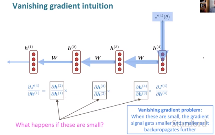
(A sketch of) a proof of this problem

What follows is a basic sketch of a proof that this occurs. Suppose our nonlinearity were just the identity function. When we calculate the partials of the hidden state w.r.t. the previous hidden state, we can use the chain rule. Since σ is the identity function, the σ goes away, and only the first term involves h at time (t-1), so the later terms go away, and our gradient ends up as Wh.

What about figuring out the partial some time away, the partial of time step i w.r.t. j? We end up with the product of the partials of successive time steps. Each of those is Wh, so we get Wh raised to the l'th power. If Wh is "small", this term gets vanishingly small as our sequence length increases.

A matrix is "small" if its eigenvalues are all less than 1 (a sufficient but not necessary condition). We can rewrite the partials of Wh^l using the eigenvectors of Wh as a basis. If we do that, we end up getting the eigenvalues raised to the l'th power, which approaches zero as the sequence length grows.

In reality σ is a nonlinearity, hence why this is just a sketch of a proof.

If we look at the influence of time steps far in the future on the representations earlier in the sentence at time t. The gradient signal from far away is lost because it's much smaller than the gradient signal from close-by. These simple RNNs are very good at modeling near effects, and bad at modeling long-term effects.

An example

Suppose we have a long piece of text:

"When she tried to print her tickets, she found that that the printer was out of toner. She went to the stationery store to buy more toner. It was very overpriced. After installing the toner into the printer, she finally printed her ___."

As a human we know that the answer is "tickets". For an RNN to learn from this training example, it would have to carry the dependency between "tickets" on the seventh step all the way to the target word "tickets" at the end. The gradient update is sent backwards through all the hidden states, but the gradient signal will be too weak to learn that dependency. In practice, the model is unable to predict similar long-distance dependencies at test time.

Exploding gradients

If a gradient becomes too big, then the stochastic gradient descent (SGD) update step becomes too big. Remember that the update is the product of the learning rate and the gradient. The parameter update can be arbitrarily large. This can cause a bad update where we take too large a step and reach a weird and bad parameter configuration (with a large loss). In the worst case, this will result in Inf or NaN in the network and we'll have to restart training from an earlier checkpoint.

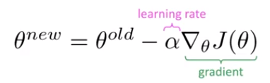
The solution to this one is gradient clipping. If the norm of the gradient is greater than some threshold, scale it down before applying the SGD update. We choose some reasonable number, commonly 20 or so, and scale the gradient down if it is above that threshold: moving in the same direction but taking a smaller step.

But how can we fix the vanishing gradient problem? In a vanilla RNN, the hidden state is constantly being rewritten. It's being changed in a multiplicative manner by multiplying it by Wh and putting it through a nonlinearity. If we could more flexibly maintain a separate memory, this would allow us to preserve information.

Long Short-Term Memory RRNs (LSTMs)

This is a type of RNN proposed in 1997 by Hochreiter and Schmidhuber as a solution to the vanishing gradients problem (but this was missing a critical part, the forget gate, until Gers et al. (2000)).

On step t, there are two hidden vectors: a hidden state h(t) and a cell state c(t). (These are named a bit strangely; in some sense the cell state is more like the hidden state of an RNN.) Both vectors are of length n. The cell stores long-term information, much like RAM in a computer. The LSTM can read, erase, and write information into the cell. The selection of which information is erased/written/read is controlled by three corresponding gates, which are also vectors of length n. On each time step, each element of the gate vector is a probability between 0 (closed) and 1 (open), to specify how much we erase/write/read. The gates are dynamic: their value is computed based on the current context.

LSTM equations

We have a sequence of inputs x(t), and we will compute a sequence of hidden states h(t) and cell states c(t). On time step t, we compute the gate values using an equation identical to the equation for simple RNNs. The forget gate controls what is kept vs forgotten from the previous state. The input gate controls what parts of the new cell contents are written to the cell. The output gate controls what parts of the cell are output to the hidden state. We use the logistic function to bound this to a probability distribution. Each gate has its own parameters: the forget gate has a forgetting weight matrix W, a forgetting bias, and a forgetting multiplier of the input.

Then to calculate the new cell content, we calculate a candidate update using the same simple RNN equation (but with a tanh nonlinearity, which is balanced around 0). We want to remember some, but likely not all, of the contents of the cell from previous time steps, and store some, but likely not all, of the value that we calculated as the new cell update. We take the previous cell context's Hadamard product (multiplying elementwise) with the forget vector, plus the Hadamard product of the input gate and the candidate cell update. For the new hidden state, we calculate which parts of the cell to expose in the hidden state with the Hadamard product of the tanh of the cell and the output gate. This is put through the softmax layer to generate the new output of the LSTM. All of these are vectors of the same length n.

The candidate update and the forget input and output gates have a very similar form, and none depend on each other, so all four can be calculated in parallel. The gates are learned - each W, U, and b is simultaneously trained by backpropagation.

Now let's look at the traditional visual representation of an LSTM.

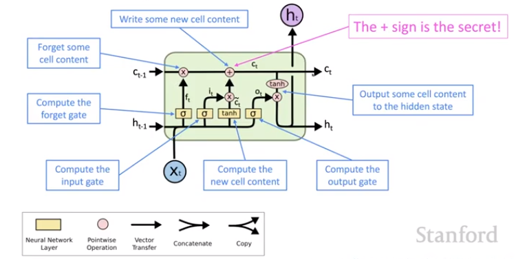
The cell state from time step t-1 is passed directly through to be the cell state at time t with only a little change - some is being forgotten by the forget gate, and something is added to the cell. Note the plus sign: new information is being added with +. This is the secret to the LSTM. Modifying hidden state via multiplication, as in the vanilla RNN, makes it difficult to learn to preserve information in the hidden state over a long period of time. It's very easy to store information in the cell (and delete it via the forget gate). (Note that the times symbol x in the above diagram is the Hadamard product, not a matrix multiplication.)

Standard practice with LSTMs is to set the forget gate to a 1 vector (forget nothing), and then let the model learn when to forget. In practice, LSTMs can preserve information for about 100 time steps rather than about 7 for a vanilla RNN. This is enormously useful for many NLP tasks. LSTM doesn't guarantee that there are no vanishing or exploding gradients, but it does provide an easier way for the model to learn long-distance dependencies.

The name comes from the idea that the hidden state of an RNN is equivalent to human short-term memory, but it was a very short short-term memory. LSTM refers to a "longer" short term memory.

Real-world success

From their inception in 1997-2000, it took until 2013-2015 for LSTM to start achieving state-of-the-art results. Successful tasks include handwriting recognition, speech recognition, machine translation, parsing, and image capturing, as well as language models. LSTMs became the dominant approach for most NLP tasks.

As of 2021, other approaches such as Transformers have become dominant for many other tasks.

More on vanishing and exploding gradients

Vanishing and exploding gradients are not just a problem for RNNs. All neural architectures, including feed-forward and convolutional, can experience this problem, especially very deep ones. Due to long sequences of applications of the chain rule, the gradient can become vanishingly small as it backpropagates, which makes them train very slowly. There has been a lot of effort to come up with new architectures that allow more efficient learning in deep networks. A common way to do that is to allow more direct connections (thus allowing the gradient to flow).

One example is residual connections, also known as ResNet, whose default behavior is to preserve the input. There are also dense connections, also known as DenseNet, which adds skip connections forward to every layer. Another example is highway connections, also known as HighwayNet, which is similar to ResNet, but adds an extra gate deciding how much of the input to send along the highway versus how much to put through a neural net layer. HighwayNet is inspired by LSTMs but applied to deep feedforward or convolutional networks.

Although vanishing/exploding gradients are a general problem, they are particularly unstable in RNNs due the repeated multiplication by the same weight matrix.

In practice it is essentially always preferable to use an LSTM over a simple RNN.

Bidirectional RNNs

For the sentiment classification task, we can run an RNN (say, an LSTM) over a sentence and take the hidden state at each step as the representation of that word in context. However, this representation only contains information on the left context (prior time steps). "Red wine" means something very different from "red light".

We can have a second RNN (with completely separate parameters learned) and run it backwords along the sentence. Then we concatenate the hidden for the word from the first RNN with the second RNN to get an overall representation of the word in context (both left and right).

This is so common that people use a bidirectional arrow between each word to draw this architecture.

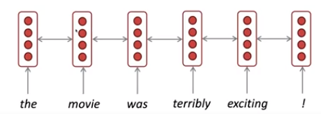
Note that bidirectional RNNs are only applicable if we have access to the entire input sequence. They are not applicable to language modeling, which necessarily has only the preceding context. But if we do have the entire input sequence, bidirectionality is powerful, and by default a good thing to use.

For example, BERT (Bidirectional Encoder Representations from Transformers) is a powerful pretrained contextual representation system build on bidirectionality. We will learn more about BERT soon.