Basics of Recording, Analysis and Data Export - articulateinstruments/AAA-DeepLabCut-Resources GitHub Wiki

Contents

1. Welcome to AAA
2. Understanding the AAA user interface
3. How to create a new project
4. How to record new data
5. How to synchronize audio, ultrasound and video
6. How to annotate regions of data with labels
7. How to fit splines to data
   • Different types of Spline
   • How to prepare video data for splining
   • Fan Splines in polar coordinates
   • Tracking the Hyoid and Mandible
   • 2D Splines in euclidean coordinates
   • Batch splining many recordings at once
   • Editing many existing splines at once
8. How to analyse and measure data, and create live graphs
9. How to export your data and analyses, and create data visualisations
10. How does AAA manage data?

---

Welcome to Articulate Assistant Advanced (AAA)!

This guide will walk you through making your first recording and analysing it. For examples, we will follow Alice as she uses AAA with an ultrasound system, camera and microphone to record a participant speaking some sentences, then analyses her data using splines and exports her results.

If you are using equipment supplied by Articulate Instruments, you can read this guide on how to set up your hardware correctly before you begin.

Understanding the AAA user interface

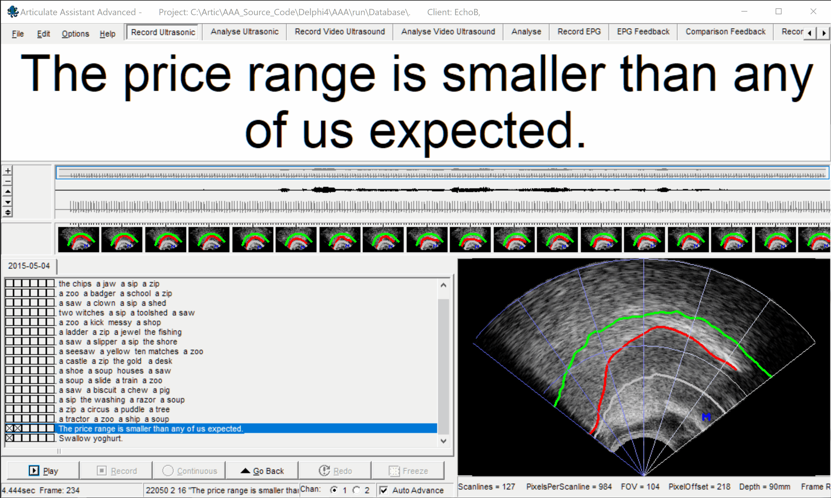
When you first start AAA, it will probably look something like this:

So what are we looking at here? AAA uses a simple drag-and-drop system to clip together useful tools and displays into one big window we can work with easily. In the above image there are 5 tools present:

• Prompt List (Used to create and curate prompts and load recordings)
• Ultrasonic Display (Shows a live readout of the ultrasound or the recorded ultrasound data)
• Audio Timeline (Shows a live readout of the audio waveform or the recorded audio data, which you can click in to navigate)
• Ultrasonic Timeline (As above, you can click and drag in this timeline to navigate a recording)
• Menu Bar (provides access to many functions and tools, and shows a list of task-windows)

You can click on the image above to see labels showing each tool.

[Note: The ultrasonic data recorded by EchoB, Micro, Ultrasonix and Art systems is held as raw scanline data in AAA and is distinct from the video stream which may contain camera images or images imported from other ultrasound systems.]

Creating a new project

AAA always starts in a demonstration project. It is not possible to record or import data into a demonstration project. A new project must be created (or a previously created project must be opened).

Example

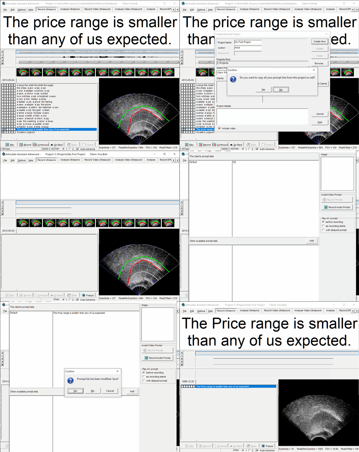
Alice is just starting her new research, so she wants to create a AAA project for it. She uses the menu at the top to select File → Create/Copy Project and then fills in the project details and the details of her participants. When she creates the project it is empty and contains no prompts. In AAA you must have a prompt to record. To create some prompts, Alice right-clicks the empty prompts-list and selects Edit → Edit Prompt List.... This process is shown below.

Recording Data

Alice is ready to record her participant. Using the prompt-list she clicks on the prompt she wishes to record and tells her participant to start speaking when they hear a beep-sound; she then presses the button at the bottom of the screen, and AAA plays a beep as it begins. The recording can then be stopped by pressing the same button again, or it will stop automatically after a time has elapsed: this automatic timeout can be set in the menu bar at the top, Options → Settings → Utterances.

[Hint: It is also possible to specify a different auto-stop time for each prompt. Simply add '/<time in seconds>' to the end of the prompt in the prompt editor.]

If Alice does not select a different prompt, she can press the record button again immediately to begin a second recording which will be stored in addition to previous recordings. All recordings she has made are displayed as filled checkboxes with an to the left of each prompt. She can click on each of them to load the corresponding recording for review or for analysis. After Alice has shown the recordings to her participant, she clicks on the text of a prompt to prepare AAA for a new recording.

Alice decides to move on to her next plan, which is to record simultaneous ultrasound, audio and camera data; she has all 3 recording devices correctly set up but AAA is not showing any camera data. This is because AAA does not currently have any camera video related tools and displays visible, so Alice changes to a different task-window by using the horizontal row of Task Windows at the top of the screen and choosing Record Ultrasonic plus Video.

This Record Ultrasonic plus Video task-window contains tools and displays we are familiar with from before: the prompt list, prompt display, ultrasound display and timelines are present as before, but now in addition we have a video display and a video timeline too. AAA could show every available tool and display simultaneously but there are so many that it would be very cluttered and hard to use, so by using task-windows we can show only the tools and displays we need for the task we want to do. If you ever want to make your own task-window because you're not satisfied with the existing ones, or if you just want to modify an existing one to suit your needs better, you can do so easily using the task-window designer.

Alice's recordings from earlier are still present in the prompt list. To keep things organized, Alice decides to make a separate prompt list for her simultaneous ultrasound, audio and video data, so she edits the prompt-list again by right-clicking it and this time she uses the menu at the top to select List→New... and creates a new empty list. She then uses the text box to the right to type in her new prompts, with each prompt on a new line, and presses OK when done. The recordings from earlier are still present, because those recordings are attached to this client (participant). Alice now selects a new prompt in the list by clicking on its text, and presses .

Synchronizing data

Alice has finished some recordings of simultaneous ultrasound, audio and camera video data, and now she wants to synchronize them exactly. Because she has been using the Micro research system to record the data, she has her recording hardware wired up with a SyncBrightup and a PStretch: these send signals to AAA which allow it to respectively synchronize video and ultrasound data to the audio recording. Options for configuring the hardware and software settings are explained in Micro Setup Guide

Ultrasound data will be automatically synchronised the first time a recording is loaded using the threshold and channel settings in the Ultrasonix setup / synchronise dialogue (found by right-click on ultrasonic display). These settings default to channel 2 and threshold 4000. Proper synchronisation relies on the PStretch pulses being present and easily visible on channel 2. If they are on a different channel or if the recording gain was low and the pulses are barely visible in the waveform display, then the channel setting may need to be changed or the threshold value lowered. An appropriate threshold level can be checked by clicking the sync button and observing if ultrasound frames line up with the audio sync pulses. However, Alice wants to export the ultrasonic data without loading each recording manually. To ensure all the recordings are synchronised she uses the batch synchronisation process in the synchronisation dialogue. She selects the date or range of dates of the recordings to be synchronised. She selects either the current client or all clients in the current project and clicks the Batch Sync button.

If the video sync signal is also recorded at the start of channel 2 then the ignore the first X ms of the sync signal should be set to X = 800.

If an ultrasonic sync signal is not present at the time of recording, the Synchronisation signal is missing checkbox can be checked and AAA will assign the ultrasound frames times according to when they are acquired. Note that soundcards usually introduce a lag which can be as much as 100ms so ideally this lag should be estimated by a tap test and then the Sync Parameters - Offset set accordingly.

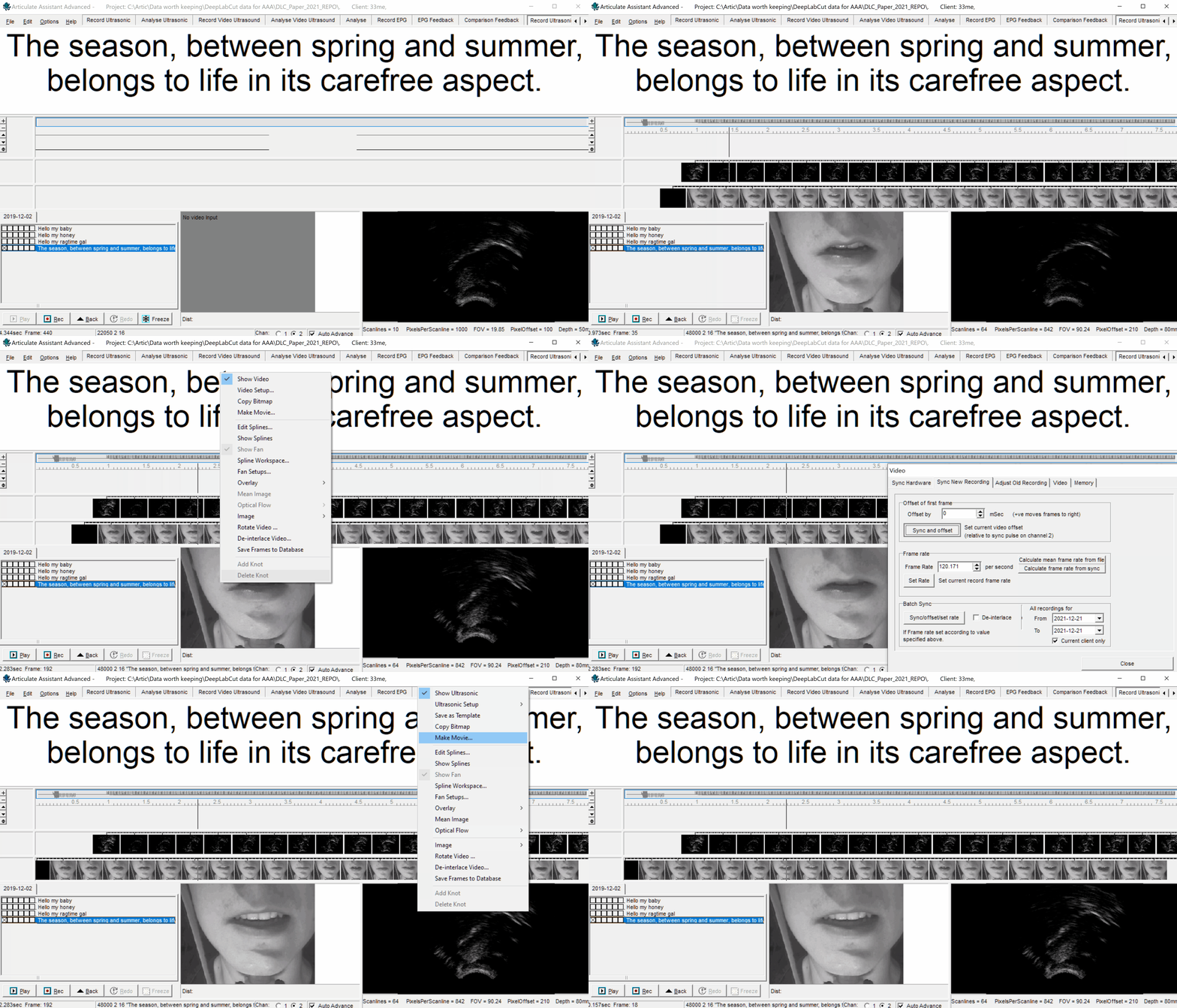
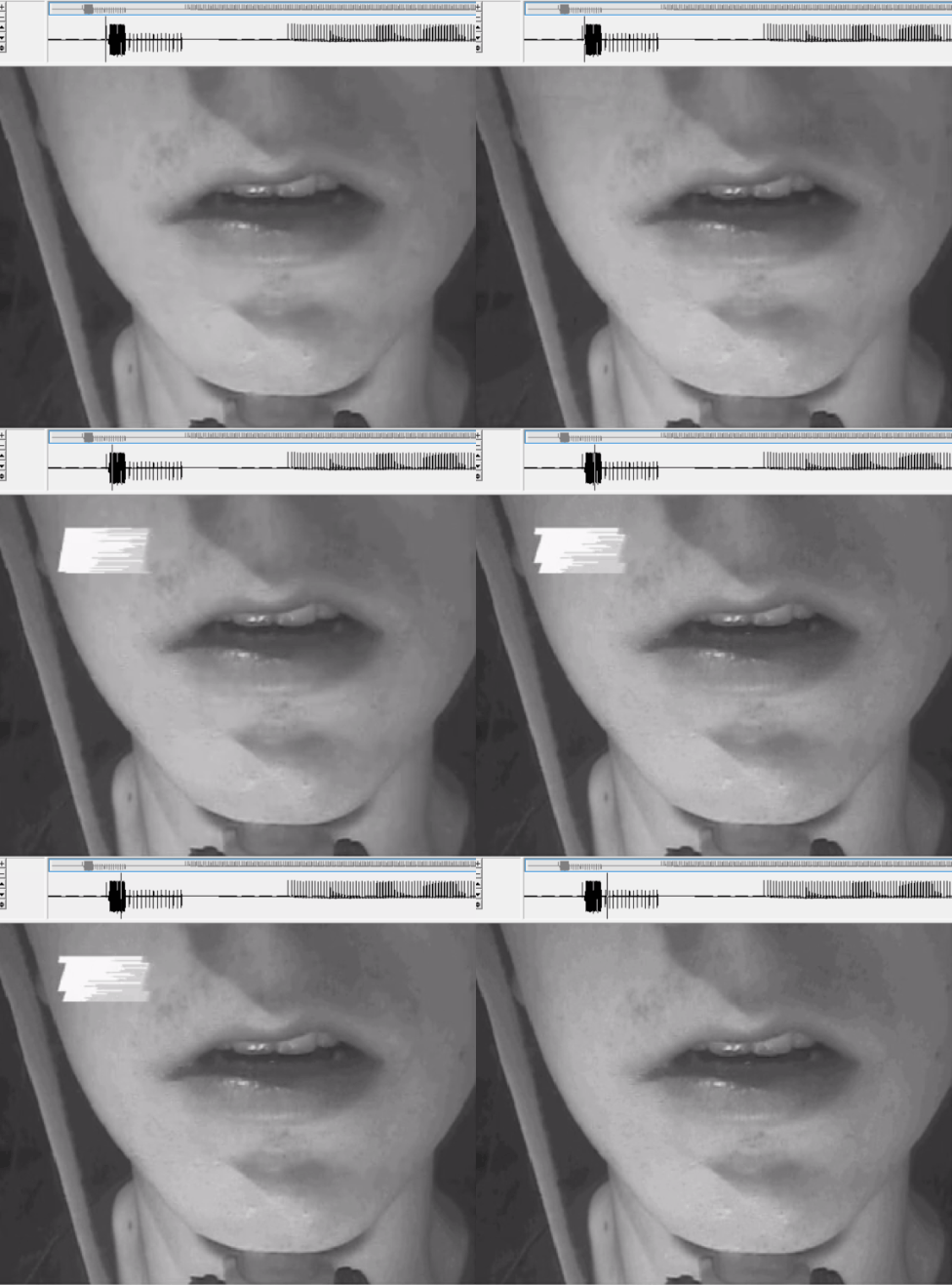
To synchronize video, Alice selects the first recording that she wishes to sync to load it, then she right-clicks on the video display and chooses Video Setup. In the tab Sync Hardware, she ensures it is set to Sync-Bright-up and the channel number is set to the audio channel with the video sync pulses. Then in the Sync New Recording tab she sets the rate to 29.97 and then clicks Sync and offset. She closes the dialog, and clicks and drags within one of the three timelines (ultrasound / audio / video) to observe that the audio beep occurs at the exact same time as the white square appears in the corner of the video. The audio timeline may only be displaying one of multiple audio channels, so you can switch the visible audio channel using the buttons on the status bar at the very bottom of the screen.

A synchronized video should briefly show a white square in the top-left corner of the video for the duration of the large pulse on the audio sync channel (one of the two sound channels), as shown below:

How does it work?

• One of the two audio channels records the microphone, and the other has an electronic signal on it.
• The signal starts with a beep, then after a pause it starts a tone.
• The video contains a small white square that appears in a corner for a few frames.
• The synchronization matches the starting beep to the white square, and then matches the ultrasound to the tone.

Batch Video synchronisation

Most often, Alice will use the Batch sync option to synchronise all the video recordings with a single click of the sync/offset/set rate button. Before she clicks this button she sets the date of the recording session or range of dates of a set of sessions and whether to process the current client only or all clients in the project. She selects the De-interlace option to separate each frame into two separate images, doubling the frame rate from 29.97 to 59.94. She sets the rate to 59.94 in accordance with this choice. Then she clicks the sync/offset/set rate button. If she chooses not to de-interlace then she leaves the rate at 29.97.

Occasionally, the synchronisation will not align the white square with the audio pulses. This may be because the sync process is restricted to looking in only the first 500ms for the sync signal. This limit can be extended by clicking the Advanced checkbox in the Sync Hardware tab and editing the Flash must be within X ms of the start setting X to perhaps 1000

Annotating Regions of Data

Alice wants to investigate phonemes for her research, so she wishes to annotate regions of her data with labels showing the phonemes. For this, she uses the annotation tool in AAA, which is a powerful tool because it allows for many operations to be done on specific annotations, for example exporting splined videos and other subsets of data for all instances of a retroflex ɻ.

First, Alice chooses a task-window which contains the Annotation tool, such as Analyse Ultrasonic plus Video. The annotation tool lists all annotations for your current project, which you can filter and edit.

To add an annotation, click and drag within the audio timeline to select a region, then either right-click within the audio timeline and select Add Annotation (and either select an existing annotation or choose <new annotation>) or click on the Add button in the Annotation tool. Next, type the label for the annotation in and then press the enter-key.

To zoom into a region of the recording to allow more precision, you can click and drag in the audio timeline and then right-click the selected region and click Zoom; to return to seeing the full recording, click anywhere in the audio timeline once so there is no region selected, then right-click and click Zoom similarly to before.

Splining data

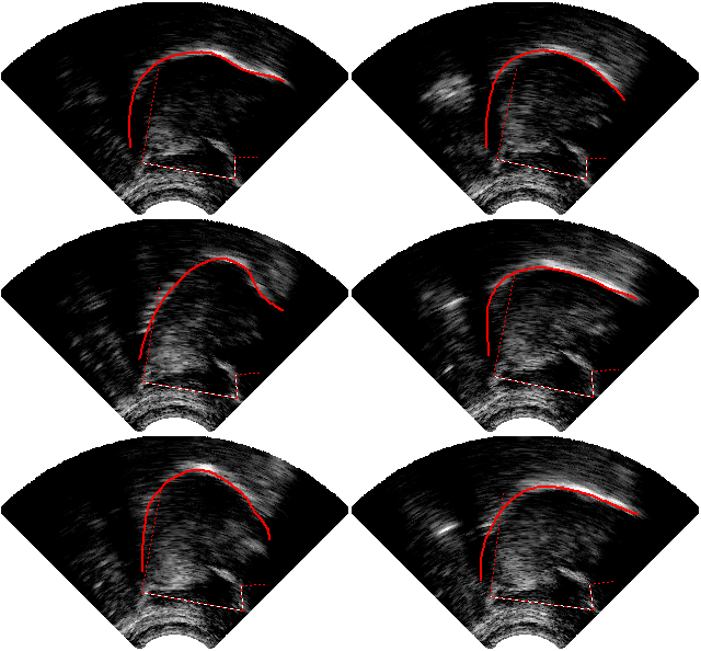
Alice wants to investigate tongue shape during specific phonemes, so she needs a way to measure the shape and position of the tongue surface. In AAA you can create splines to follow the contour of the tongue surface or the positions and movement of other anatomy, and you can either place them manually or fit them automatically.

Splines are useful for many kinds of analysis: they can interact with many features of AAA. There are three types of spline, and choosing the right one to use depends on what you want to measure:

• 2D Splines = These use euclidian coordinates: measurements are in x, y and pythagorean distances relative to the visible area.

  • 2D splines currently offer the best automatic spline fitting. It uses machine learning to avoid bright ultrasound artefacts, and estimate the tongue's position in regions shadowed by bone or where the probe has lost contact.
  • 2D splines allow for any shape, including looping back and intersecting itself.
  • Built-in analysis tools for euclidian coordinates can be performed on 2D splines, such as measuring euclidian distances and angles between the knots of two splines or calculating mean-sum-of-distances to measure similarity of groups of splines.
  • 2D splines can be used for some polar-type analysis from a moving origin, for example approximating Genioglossus muscle lengths relative to the short-tendon origin.
  • 2D splines can be used to track and compare lateral movement of objects whereas Fan splines can only track movement towards and away from the probe origin.
  • Can be automatically batch fit to tongue anatomy with built-in tools that interface with DeepLabCut and other machine learning; such tools can only fit 2D splines and cannot fit fan splines.
  • Splining of video camera data, such as in analysis of lip position/shape, is best done with 2D splines.

• Fan Splines = These use polar coordinates originating from the ultrasound probe: measurements are in angle and distance from the probe.

  • Fan splines can also be automatially fitted, but this is done using an older technique that is faster but significantly less accurate than automated 2D spline fitting.
  • A fan spline can NOT double-back on itself, such as can occur at the tongue root or for the shape of the tongue tip in a retroflex ɻ, but a 2D spline can.
  • Fan splines can be used with the Spline Workspace (a suite of tools for comparing and analysing tongue-surface splines).
  • Fan splines can be manually drawn on the tongue surface very easily and quickly.
  • Can be automatically batch fitted to the tongue surface quickly with built-in tools in AAA edge tracker.
  • The built-in analysis tools for polar coordinates can be performed on fan splines, such as measuring how the closest point between the tongue surface and the roof changes over time. can be exported in polar or Euclidean co-ordinates for analysis in other software

Both types of spline can be used for shape-based analysis, for example calculating the dorsum excursion index (DEI) or the number of inflections (NINFL), and both types of spline can be manually adjusted at any time.

• Fiducial Splines = These use euclidian coordinates like 2D splines, but a fiducial only has 2 points, so is always a single straight line.

  • Fiducials are usually used as references for measurements involving other splines, for example acting as a ruler against which to measure something, a boundary to be crossed, or to define a frame of reference.
  • A fiducial can be set to the bite-plane and used to rotate exported co-ordinates so that the x-axis is set to the Fiducial and the origin is set to the fiducial origin.

You can convert Fan Splines into 2D Splines, and convert 2D splines into Fan Splines, but doing can be partially destructive to your data. 2D splines can double-back on themselves but Fan splines cannot: converting 2D to Fan will preserve only the closest spline surface to the probe origin. Furthermore, there cannot be more or less knots than fan lines, so additional knots may need to be created at arbitrary radii, and knots beyond the range of the fan will be removed. Fan splines always have a number of knots equal to the number of fan lines, which is a fixed value of 42, but 2D splines can have any number of knots from 2 to 50. When converting Fan to 2D you will be prompted to choose the number of knots: if the number of knots you choose differs from the number of fan lines, the knot positions will be calculated as intelligently as possible, but choosing fewer knots than fan lines will still be fundamentally destructive to the resolution of your data. Because of all these reasons, it is recommended that you carefully consider the data analysis you wish to perform before choosing whether to use Fan Splines or 2D Splines.

Splining: 2D Splines

In AAA you can automatically fit 2D splines using powerful external tools. AAA natively supports DeepLabCut, a free open-source state-of-the-art machine learning tool, which can automatically fit splines using DeepLabCut entirely within AAA.

🡒 A simple tutorial on how to use DeepLabCut in AAA can be found here 🡐

You can also fit 2D splines using any other external tool of your choice and easily import them into your AAA project.

Splining: Fan Setup

Fan grids have two main functions

• Defining the origin and angular extent of the polar grid
• Setting the scaling from pixels to real-world co-ordinates (mm)

If you have recorded your data with a Micro, EchoB or Art system then the fan grid and origin extent and scaling are automatically calculated. When you add a new set of fan splines to a recording simply select the fan setup with a tick next to it. You can skip to the next section of this tutorial here.

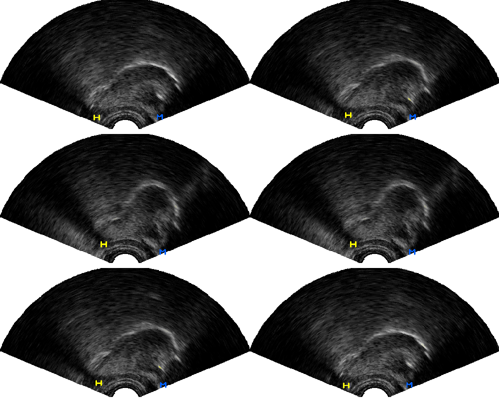
If you are using an ultrasound system which connects to AAA by video input (for example a Mindray 6600 ultrasound system) or you have imported *.avi files of ultrasound data then you will need to set up a Fan manually. This is how you inform AAA where the probe origin is relative to the image, and what the field of view of the recorded data is.

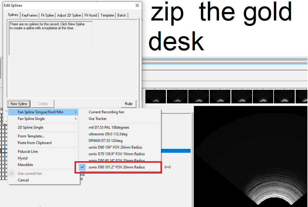
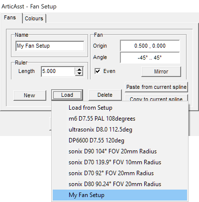
First, check if a fan already exists and is invisible: right-click on the video display and you will see an option called Show Fan. If that does not have a tick to the left of it, then click it to make any existing Fans visible. If there is no Fan present, you can proceed to set one up: right-click on the video display and select Fan Setups. Click on Load: many different ultrasound systems have presets present here, and you may find your ultrasound system already listed, which you can then click to set up the fan for it instantly.

• D = Depth (eg. D90 = 90mm depth).
• FOV = Field of View (eg. 104° FOV or 104deg = 104 degrees).
• Radius = The distance from the probe origin (where the fan converges) to the surface of the probe.

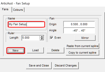
If you cannot find a preset that matches your equipment, please instead click on the New button to the left to create your own preset. Name your new preset with the Name field above.

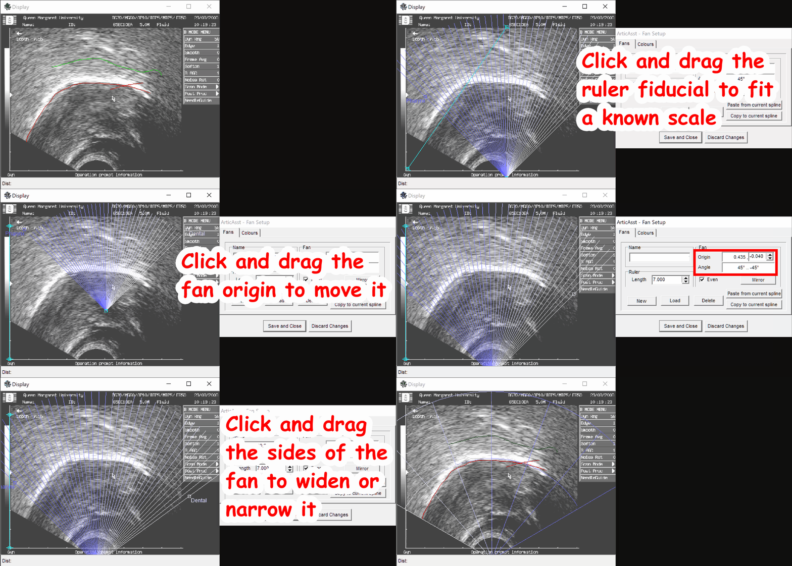
The Fan Setup display shows the ultrasound image with a fan overlaid on the image, and you can manipulate the fan by clicking and dragging the anchor points: one at the bottom controls the fan origin, and there is an additional anchor on each side of the fan half-way up which controls the angle on that side, and you can type in specific values on the right side of the dialog. You also need to tell AAA what the scale of the image is (eg. 5cm from top to bottom): the ruler is a straight line on the image with an anchor at each end which you can drag around, for example lining it up with a scale overlaid on the image by your ultrasound hardware. You can then type the distance it corresponds to on the right; the units of measurement are your responsibility to define, remember, and be consistent with in your project.

Splining: Fan Splines

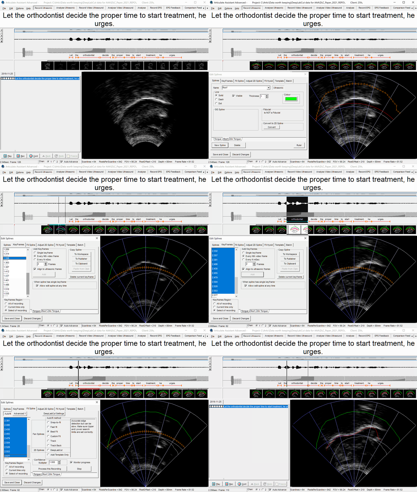
Splines are be created and edited using the Edit Splines dialog, which you can open by right-clicking anywhere on an ultrasound or video display and clicking Edit Splines.... Splines are always specific to each recording, so if you create a spline for one recording it will only be present on that recording, but there are tools to create, edit and fit splines to many recordings with a single key click, and those tools will be discussed later in this tutorial.

The Splines tab at the top left of the dialog shows the page where you can create new splines or change the appearance of existing splines.

If any splines exist for a recording they will always appear as tabs along the bottom of the dialog. Any tools and properties on each page that you can edit apply only to the spline currently selected unless otherwise specified.

Alice wants to analyse the shape of her participant's tongue, but at the moment she's only interested in certain words in the recording. She decides to create a spline and fit it to the sub-region of her latest recording where the word of interest is spoken. To do this, she needs to first create splines for her ultrasound data so she begins by right-clicking the ultrasound display and selecting Edit Splines.... There are no splines currently in her recording, so she clicks New Spline. Here, there are many options. She can create either Fan splines, 2D splines or fiducials.

Alice wants to perform analyses in polar coordinates, so she decides to use Fan splines because they are defined in polar coordinates, unlike 2D splines which use euclidean coordinates. (She does not use a fiducial spline either because a fiducial is a single straight line between two points, used as a reference point for other analyses, and so is unsuited to contouring around a tongue surface.)

When creating a spline, one of the options is to create Tongue/Roof/Min Tongue: many fan-spline related features of AAA are designed to work especially quickly and easily with this special trio of splines. Roof and Min Tongue should define the upper and lower limits in the mid-sagittal plane within which the tongue will stay. If you want to use automatic tongue tracking, you should fit Roof and Min Tongue manually by selecting each of them in turn and clicking and dragging the mouse-cursor in the ultrasound display to draw their shape. You can still click and drag in the timeline to navigate through your recording, which may help you to see the limits of the tongue's movement over the recording (you can do this without needing to close the Edit Splines dialog).

You can create splines that stay constant throughout a recording and you can create splines that change over time. Every spline has Keyframes, which can be seen in the Keyframes tab at the top. A keyframe is a point in time where a spline has a particular shape. Keyframes are listed on the left as numbers, where each is the number of seconds since the start of the recording at which that keyframe exists. You can manually create keyframes at specific time points in the recording by clicking in the timeline for the recording and then choosing Single keyframe and clicking Add. You can also create many keyframes at once by click-drag selecting a region of the recording in the timeline, or double-clicking an annotation, and then choosing Every Nth video frame or Every N mSec and clicking Add. Any two spline keyframes with a gap of time between them will fill that gap by linearly interpolating between the shapes at each keyframe, eg: | → ( → C

A spline that you want to stay constant throughout a recording should have only one keyframe (which should be listed on the left as a single number). In the time before a spline's first keyframe, it will have the same shape as has in its first keyframe, and likewise in the time after a spline's last keyframe it will have the same shape as in its last keyframe.

Alice creates keyframes for the Tongue spline by selecting her region of interest in the timeline, then selecting Every Nth video frame and clicking Add. She leaves Roof and Min Tongue with only 1 keyframe each, as they were created, because she wants them to stay constant throughout the recording.

Next, Alice clicks on the Fit Spline tab to choose an automatic tracking method appropriate for fan splines. There are multiple options available:

• Best Fit: Searches along each fan line, from the probe origin out to the most distal points on the fan, and searches for the brightest edge. The parameters for how it determines the brightest edge can be selected in the Advanced 1 tab at the top, but it is advised to leave the settings at their defaults, as they have been carefully calibrated to give good results.
• Fast Fit: This works exactly the same way as Best Fit but performs its calculations on a lower resolution of data, so processes significantly faster but gives slightly less accurate results.
• Snap-to-Fit: Searches for a bright edge in the same way as Best Fit, but only looks near the spline's current position/shape. This is particularly useful if you want to manually draw the spline shape, as you can then use Snap-to-Fit to contour it exactly along a nearby bright edge. In the Advanced 1 tab you can choose how far each knot should try to search from its current position.
• Track: This only works when splining more than one keyframe at a time. It uses Snap-to-Fit, but instead of using the position/shape of the current spline keyframe, it uses the position/shape of the spline in the previous keyframe as the seed to calculate the new keyframe from. This can be useful to stop bright areas which briefly appear in the ultrasound image from attracting the spline. Track Back does the same, but progresses in the opposite direction, starting at the chronological end of the recording and working back towards the beginning.

Best Fit and Fast Fit make important use of the special Roof and Min Tongue splines because they define the limits within which the search for a bright edge will occur. This is important to help the algorithm find the tongue surface and prevent it from misinterpreting other bright areas of the ultrasound image as being part of the tongue surface.

Next, in Keyframes Region in the bottom-left Alice either chooses Select of recording which would cause tracking to be done on the selected keyframes (either as selected in the timeline or as selected in the list on the left), or she chooses All of recording which would cause tracking to be done on all currently existing keyframes. She then clicks Process this Recording. When the tracking finishes, Alice selects the Tongue spline and selects individual keyframes in it and makes some manual adjustments where she thinks the automatic tracking has made mistakes.

Splining: Hyoid and Mandible

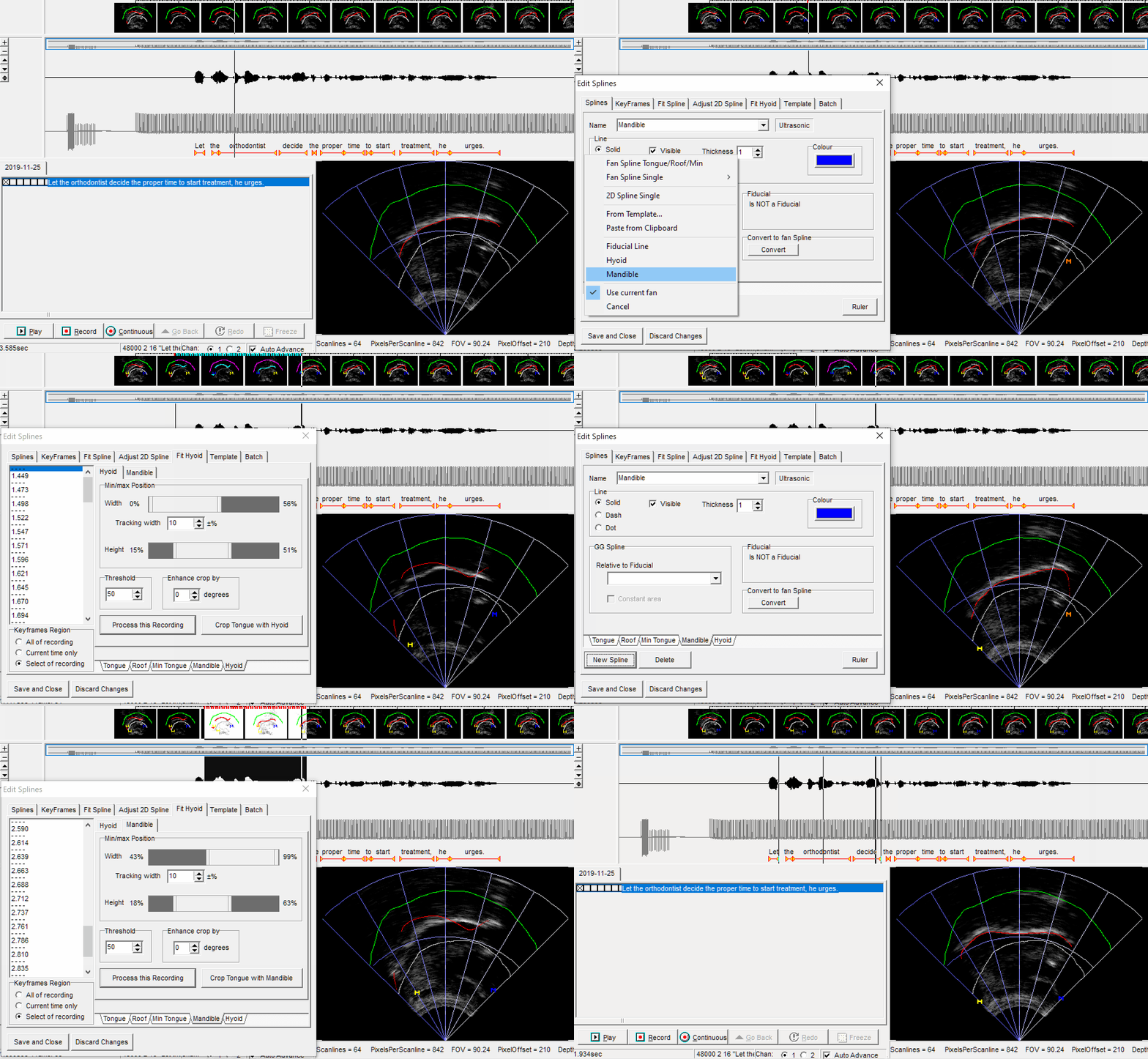
In addition to splines, you can also automatically track the hyoid and mandible:

You can create a Hyoid label and a Mandible label using the same button to create a new spline. Each of these labels marks a single spatial point, and you can automatically fit them to the data in a very similar way as you can fit splines, using the Fit Hyoid tab.

Alice reconsiders the analysis she wishes to perform on her data and decides to use 2D splines instead. She doesn't want to destroy the splines she's made so far. To tidy the image she temporarily hides the fan splines from view. On the Splines tab she selects each of her existing Splines one-at-a-time and unchecks the Visible box .

Batch splining many recordings

Once you are familiar with how to manually and automatically fit splines for individual recordings, you can try Batch Splining.

Batch Splining does the same process as you did to fit a spline for one recording, but repeats it automatically for as many recordings or annotations as you want across any number of Clients within a project. This means you only have to choose the splining settings once at the start, then it will fit all the specified splines according to those settings.

You can use this with either Fan Splines or 2D Splines; the process of using each is a bit different. To learn how to batch fit 2D Splines (which can be done using cutting-edge machine learning for more accurate results), please read this short tutorial. For Fan Splines, continue reading below.

Batch Fan Splining works by first defining one or more splines to act as a template: you only do this once, and then when you run the batch process each of these template splines will be automatically duplicated once for every recording being processed. Each of these sets of duplicated splines will then be used as the starting point from which to run the chosen tracking algorithm within each recording. So each time the batch process loads a new recording, it will paste the copied splines once, and then use them as the initial state of the splines when it runs the tracking algorithm for the recording.

The special splines called Roof and Min Tongue, as explained earlier, define the upper and lower limits within which the algorithms will try to search for the tongue. This is especially important here because we want the spline to fit the tongue surface most correctly in each recording, and to do that those upper and lower limits need to include the full range of tongue movements but also exclude as many bright areas as possible which aren't part of the tongue surface. The challenge is that we need to create one position/shape of Roof and Min Tongue which will be used as the limits for every recording. (You can make exceptions where you use a different Roof and Min Tongue for individual recordings in your batch, and this will be explained next.)

The process may seem complicated, but it will become clearer as we walk through an example.

Alice plans to batch spline all the recordings she has made so far of her participant. She knows that she will need to define the Roof and Min Tongue as limits for tracking all her recordings, so she loads a few of her recordings and looks through them to familiarise herself with the limits of her participant's tongue movements. Alice chooses an arbitrary recording of her participant and opens the Edit Splines dialog by right-clicking on the ultrasound display. She clicks New Spline and selects Fan Spline Tongue/Roof/Min to create a Tongue, Roof and Min Tongue spline. Alice selects each of Tongue, Roof and Min Tongue in turn and clicks and drags her mouse cursor on the ultrasound display to draw the shape she wants for each, according to where she wants the upper and lower limits for all recordings. The 'Tongue' should be in a neutral position below the 'roof' and above the 'MinTongue' splines.

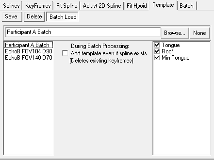
Alice now needs to save these Tongue, Roof and Min Tongue splines as a template to be used later in batch processing. Alice clicks on the Template tab at the top of the dialog. Here, she can see a list of all the splines currently in this recording. She clicks on the checkboxes to select Tongue, Roof and Min Tongue and she leaves all other splines unchecked, then she types in a name for her template into the field to the left: she chooses a name that will help her remember what this template is for. She then clicks Save. (You can also Save to File... and back up the saved template or move it to other computers, for example sending it by email).

Now that Alice has saved her Tongue, Roof and Min Tongue splines as a template, she no longer needs to keep them as splines in the recording she made them in, and she can safely delete them.

Alice is almost ready to start the automated batch splining process, but first she needs to choose which algorithm to use. She clicks on the tab Fit Spline at the top of the dialog, and chooses an algorithm in the same way as she did for splining a single recording. There is no need to select any keyframes at this stage, and any keyframe selections here will not be used. She does not click on the button to process the current recording.

Next Alice clicks on the 'Fit Spline' tab at the top o the dialog and selects the 'Track' option from the 'FanSplines' autofit methods.

Next, Alice clicks on the Template tab again at the top of the dialog. This time, she clicks on the Batch Load sub-tab near the top. Here, Alice can see on the left a list of all templates she has previously saved, including her template she has just recently saved from her Tongue, Roof and Min Tongue splines. She clicks on it in the list on the left, and on the right those Tongue, Roof and Min Tongue splines appear. Alice wants to provide the Tongue, Roof and Min Tongue splines to the batch process to define the tongue initial position and upper and lower tracking limits, so she ensures that the checkboxes for the three splines are ticked on the right by clicking on them. (If you want to load a template from a file instead, you can click on the Browse... button and select the appropriate file on your computer.)

Next, Alice clicks the Batch tab at the top of the dialog, and then the Choose Recordings sub-tab beneath it. This is where Alice needs to specify which recordings should be automatically processed.

First, Alice must choose whether the automatic batch splining should process each selected recording in its entirety, or only spline certain annotations (which could be all annotations if that is desired). She wants to process entire recordings, so she clicks on the Recordings button.

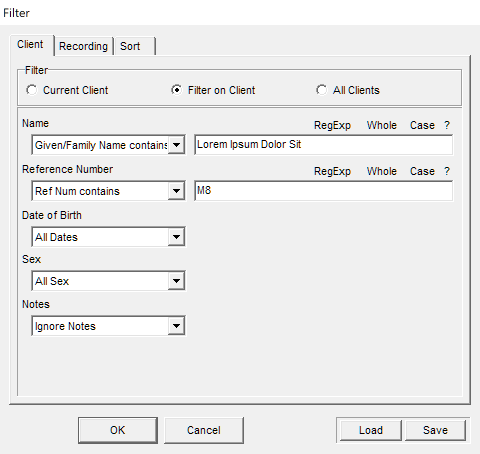
Next, she clicks on Change Filter. This shows a new dialog with 3 tabs: Client, Recording and Sort.

Alice clicks on each tab in turn and selects the options available to specify what data she wants the batch splining to operate on. She wants to batch spline all the recordings for her "Participant A": to do this she could either choose Current Client if she had a recording from "Participant A" currently loaded in AAA, or alternatively she could click Filter on Client and use the options to specify the client she wants. Furthermore, because Alice wants all the recordings for "Participant A" to be batch splined, she chooses All Recordings. The Sort tab defines the order in which the recordings or annotations will be processed, but does not affect which data gets processed. Alice clicks OK at the bottom of the dialog to close and save her choices.

The conditions that you can specify in the three tabs combine both within each tab and also across tabs with 'AND'. Regular Expressions are parsed by the TRegExpr library which supports most but not all modern regex functionality.

The large white box on this dialog page now shows a list of all the recordings that Alice has specified. She visually inspects the list to double-check that it looks correct.

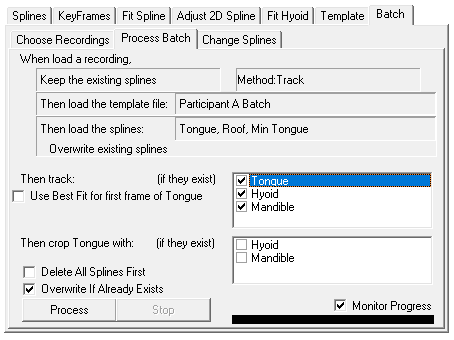
Next, Alice clicks on the Process Batch sub-tab at the top. This page shows a summary of all the choices she's made so far.

Alice wants to track the tongue. She's not interested in the Hyoid or Mandible at this time, but she checks the boxes to track them anyway, so she can make them invisible afterwards and they will be available if she changes her mind. The Crop tongue with selection allows you to make all spline knots to the left of the hyoid and to the right of the mandible (respective to the probe origin) automatically have confidence of zero (and thus be invisible), which may be useful in certain research projects. Alice leaves them unchecked.

It is now time for the automatic processing: Depending on the amount of data you have chosen to be automatically batch processed, and depending on the power of your computer's processor, this might take a long time. Tracking on video data (including ultrasound systems that provide video data to AAA) is significantly slower to process than raw ultrasound data. The first time you process, it is recommended to enable Monitor Progress in the bottom-right, which slows down processing but shows you a live visualisation of the automated spline fitting so you can verify it's doing what you want. If you have a very large amount of data to process you might then want to disable Monitor Progress if you are satisfied that it's doing what you expect.

There are many factors that affect processing time so it's very hard to estimate. One user of AAA might find that their batch processing is ten times faster than another user's because of differences in their computer, the nature of their data and the algorithm(s) they've chosen. The only thing you can do is try it for yourself and find out. Processing progress across all your selected data is displayed in the progress bar at the bottom of dialog, and depending on the algorithm you're using there might also be an additional progress bar showing progress through each individual recording too.

Be careful because you cannot undo any batch changes you make; it's always good practice to keep incremental backups of your work. When you are happy with all the options you have selected, click the Process button to begin.

Batch Editing many Splines at once

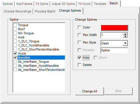
Alice has finished batch processing many recordings with a spline fitting algorithm and now she wants to make the Hyoid and Mandible splines invisible in every recording without having to do it manually. This is easy to do.

In the Edit Splines dialog, in the Batch tab at the top there is a Change Splines sub-tab near the top. This lets you change many properties of splines, including their appearance, visibility and name, or delete them.

The list on the left shows every spline for every client in your currently loaded project. You can choose to only affect a subset of your project's splines by using the Choose Recordings sub-tab above and proceeding to Filter the data, for example only affecting splines in recordings between certain dates. In the Change Splines sub-tab you can select splines on the left by clicking on their individual checkboxes, then on the right choose what you would like to change about them. You can select multiple things on the right and they will all be applied to all the selected splines on the left when you click Change All. Be careful because you cannot undo any batch changes you make; it's always good practice to keep incremental backups of your work.

Analysing and measuring data using Analysis Values

The Analysis Values system is a powerful suite of data analysis tools in AAA. It allows you to create many different measurements of recorded data and their relationships to each other. You can create and format graphs of Analysis Values and create your own mathematical formulae to modify Analysis Values or combine them.

Task Windows each contain only some of the tools and displays available in AAA. Before you start working with Analysis Values, it is recommended that you move to a Task Window that contains Analysis Value displays and graphs, by clicking on one in the menu bar at the top of the screen. All of the following Task Windows contain Analysis Value tools and displays by default and can be used to analyse any type of data:

• Analyse Ultrasonic (also contains Audio and Ultrasound displays)
• Analyse Video Ultrasound (also contains Audio and Video displays)
• Analyse (also contains an Audio display)
• Analyse Ultrasonic plus Video (also contains Audio, Ultrasound and Video displays)
• 2-Screen Ultarsound and Video (also contains Audio, Ultrasound and Video displays)

Next, in the menu bar at the top of the screen, click Options → Analysis Values... → Edit...

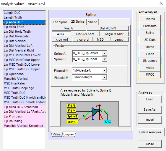
The Analysis Value dialog might look complicated when you first see it, but it's quite straightforward.

• On the left is a list of all Analysis Values that you have created in the current project. (Analysis Values are shared across all clients within a single project. If you've created a new project then it will have automatically copied all Analysis Values from the previous project you had loaded. You can easily delete a selected Analysis Value using the Delete Analysis button in the bottom right).
• The buttons on the right side of the dialog let you create new Analysis Values: Each button represents a different type of data and each contains many different Analysis Values that can be used with that data type.
• The main area in the middle lets you learn about and choose the type of data analysis to perform.

Alice is interested in the contraction of Genioglossus muscles attached to different points along the tongue's surface during production of particular phonemes. She has recorded mid-sagittal ultrasound data and has chosen to use DeepLabCut to fit 2D splines to her data. Thus, certain analyses will suit her research intents and her methods more than others.

There are many Analysis Values you can create to measure and compare different things. Every one provides its own explanation and diagram showing what it does. You can see this in the area below each Analysis Value's settings. (For example in the image above you can see the 2D Spline Area analysis is selected, and so a diagram is visible explaining the functionality of this selected Analysis Value).

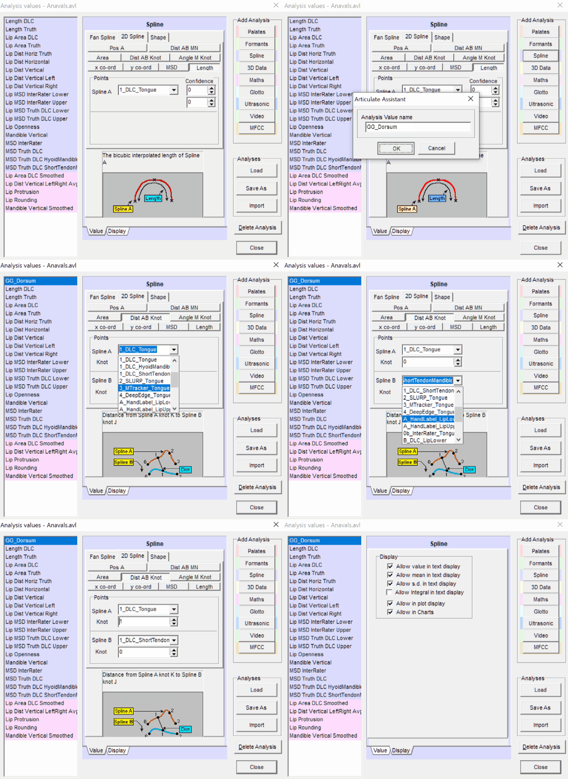
When Alice fit 2D splines to her data using DeepLabCut, she splined the tongue surface and also the hyoid, the mandible and the short-tendon. In order to measure the Genioglossus muscle contractions, she wants to measure the distance from the short-tendon to various points on the tongue surface. Because this is a measurement of spline data, she creates a Spline Analysis Value.

Alice clicks on the Spline button on the right to create a new Spline Analysis Value and she gives it an appropriate name. (If you wish to rename an Analysis Value, you need to delete it and remake it). She ensures that she has her new Analysis Value selected in the list on the left, then because she's working with 2D splines she selects the 2D Spline tab at the top, and because she wants to measure the distance between two knots (one on the tongue and one on a spline that defines the short-tendon), she clicks on Dist AB Knot to measure the distance between two spline knots. She then uses the drop-down boxes to specify the splines, and inputs the index of the specific knots (the first knot is index zero).

Alice repeats this process to create a total of 5 Analysis Values corresponding to her chosen tongue regions: Root, Body, Dorsum, Blade and Tip. Each Analysis Value she has created now measures the distance from a tongue region to the short-tendon.

After closing the dialog, the new Analysis Values become automatically visible overlaid together on line graph in AAA, showing the change in each Analysis Value over time. However, at the moment the formatting is very simple, homogeneous and hard to read. To the left of the graph, the Analysis Values present in the chart are listed.

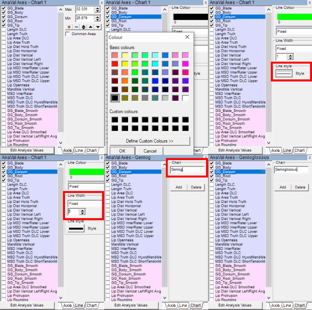
You can easily improve the appearance of the chart. Right-click on the Analysis Value names to the left and click Edit Chart.... You will see a dialog showing all Analysis Values in your project with a checkbox to the left of each. You can tick or untick them to show or hide them on the graph. To the right is the settings for the currently selected Analysis Value.

• The Axis tab at the bottom allows you to fine-tune the vertical axis. (The horizontal axis is always tied to the visible region of the recording, which you can change by clicking and dragging the mouse cursor in the audio timeline, then right-clicking within your selection and clicking Zoom; you can then drag the sides of the selected region around to expand or contract them).
• The Line tab at the bottom lets you change the appearance of the selected Analysis Value in the chart, for example changing its color, style and thickness.
• The Chart tab lets you name the current chart, and also create a new chart with the Add button. New charts will be visible adjacent to your other chart(s), which allows you to split your Analysis Values across multiple charts for clearer visualisation and comparison.

When Alice finishes making changes, she closes the dialog then refreshes the chart to ensure her latest changes are visible: You can click Options → Analysis Values... → Re-Calc Current Recording to make AAA recalculate every Analysis Value to incorprate any changes that's been made. Then, right-click on the Analysis Value chart and click Zoom and choose an option. Alice is more interested in relative comparisons than absolute ones, so she clicks Zoom → Zoom each to fit which normalises every line on the graph show its minimum as the lowest value within the visible graph area, and show its maximum as the highest value within the visible graph area.

It's good practice to make a habit of recalculating and zooming any time you make a significant change to an Analysis Value.

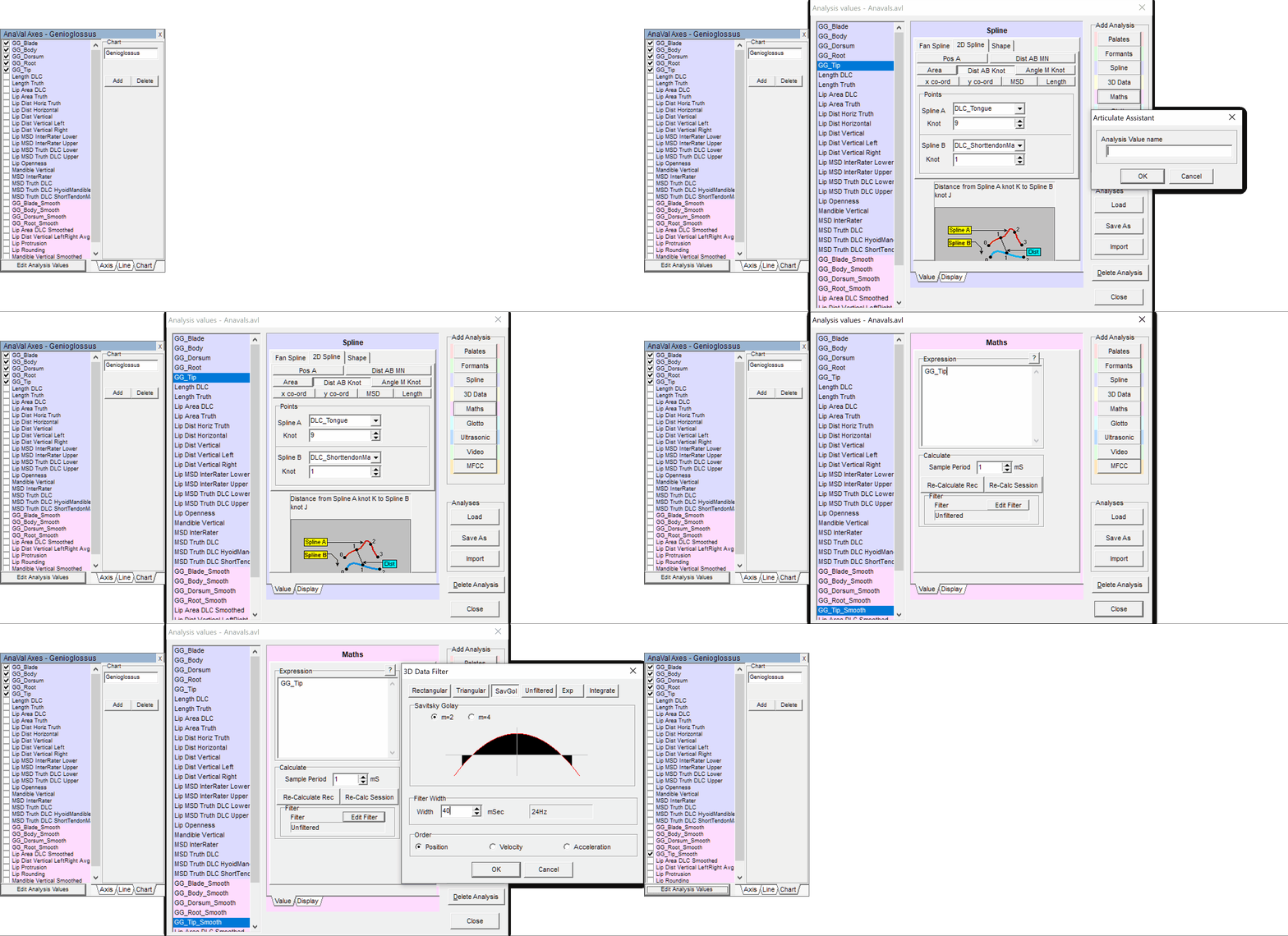
Alice has formatted the different Analysis Values in her chart to look clearer and more readable, but she's worried that the estimation error noise in the DeepLabCut splining is making it hard to see the trends. She decides to create a smoothing filter: this can be done using Maths Analysis Values.

Alice re-opens the Analysis Values dialog from the menu at the top (Options → Analysis Values... → Edit...). She creates a new Maths Analysis Value by clicking the Maths button on the right and gives it a descriptive name for its intended purpose. A Maths Analysis Value consists of a free text field where you can type in a formula.

All Analysis Values of any type must ultimately evaluate to a scalar. For Maths Analysis Values, you can see a list of all operators and functions you can use by selecting a Maths Analysis Value and clicking the question-mark (?) button near the top.

Maths Analysis Values also include an optional smoothing filter (which is applied after your specified equation resolves but before any differentiation). You can click on the Edit Filter button below your equation and choose a smoothing filter using the tabs available at the top of the new dialog.

By creating a Maths Analysis Value it will be automatically added to your existing charts, and it exists separately from any Analysis Values that are used in its equation (even if it only exists to smooth another Analysis Value). You may wish to format your new Maths Analysis Value to make it more presentable on the chart.

After trying the different smoothing filters, Alice settles on a SavGol (m=2) filter operating on a sample window of 40ms, and as such she creates a Maths Analysis Value to act as a smoothed version of each of her Spline Analysis Values. She edits the chart to show her new Analysis Values instead of her original Spline Analysis Values, and formats them to be visually easier to read.

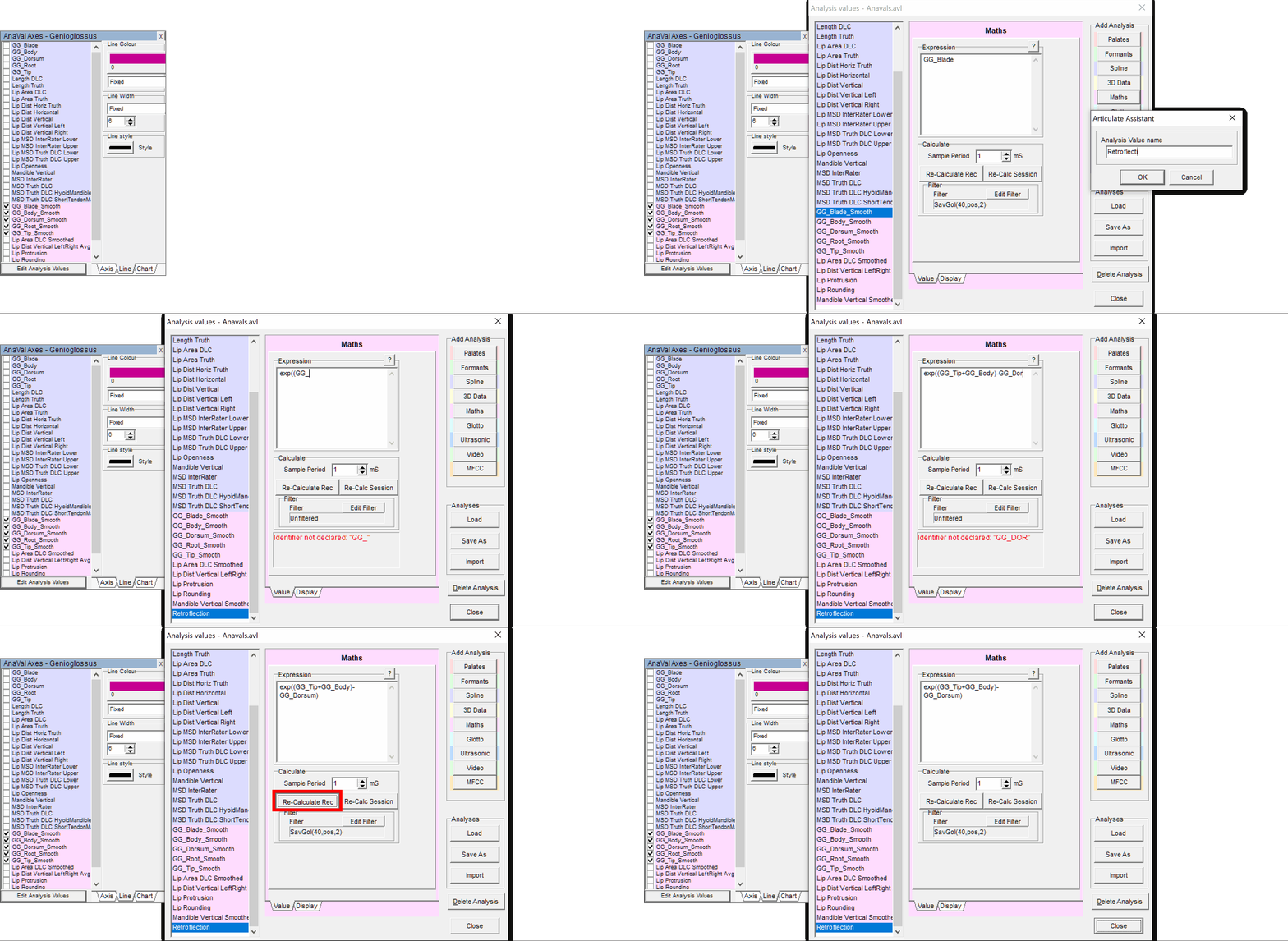
Next, Alice wishes to create a metric that describes the degree of retroflection in the tongue. This is what Maths Analysis Values are really useful for. She re-opens the Analysis Value dialog, creates a new Maths Analysis Value which she names descriptively, ands then she writes an equation for it.

In the chart editor, she uses the Chart tab at the bottom to Add a new chart, and checks the box for her new Analysis Value "Retroflection" to load it into the chart. By using multiple charts and distinct readable formatting, Alice can keep specific Analysis Values overlaid for visual comparison while keeping others separate.

Exporting Data

Alice has finished analysing her data and wishes to export her results to put in a paper. AAA provides multiple tools for exporting data in useful formats:

• "Publisher": Make visualisations of your data, such as combining labelled graphs, timelines and other information directly from your project into a single image.
• "Make Movie": Design animated videos that show multiple types of data concurrently changing over time in a clear, readable layout.
• "Export Data": Get tables of Analysis Values and raw data values as comma-separated-variable (.CSV) files for putting in an appendix or for further analysis (eg. R, SPSS, Excel).
• "Export Files": Export your raw recorded data in its entirety out of AAA for backup or for importing into other software.

Publisher:

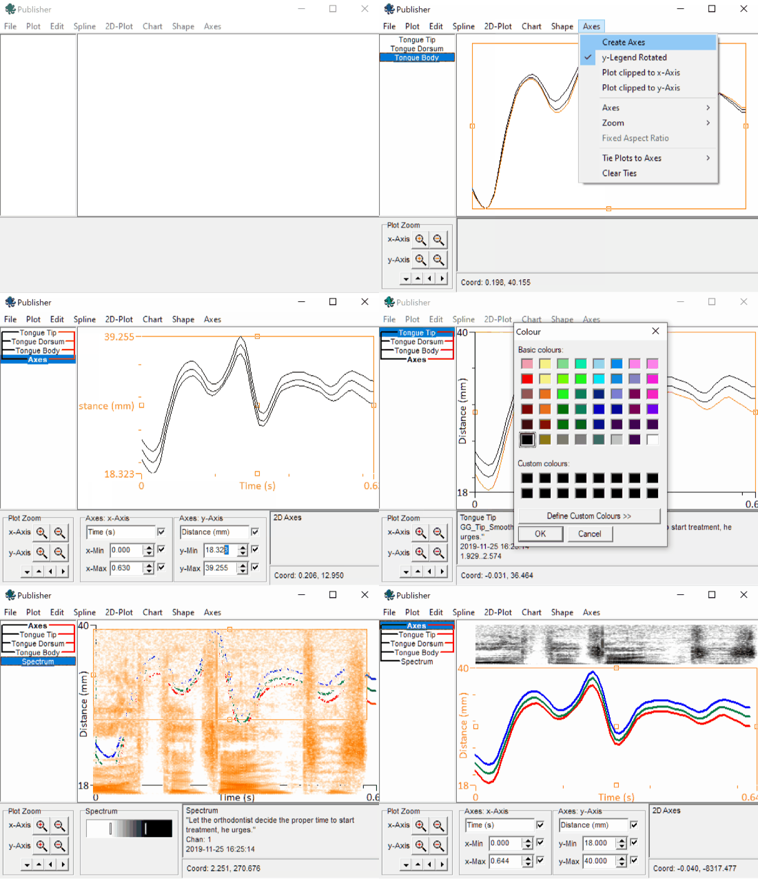
So far, Alice has used many tools in AAA to help her find interesting patterns in her data, and now she wants to present some examples of her findings. The Publisher in AAA is a fast, easy way to make plots of data and automatically keep data tied to common axes for comparison. You can arrange and format data visualisations and then export them as images to put in a document or import into other software.

You can open the Publisher from the menu bar at the top of the screen by clicking File → Publisher...

When you first open the publisher it might initially look confusing, but its controls are simple and consistently laid out.

• At the top is a row of menus you can use to load in new Elements such as data plots, labels, etc.
• On the left of the Publisher is a list of all Elements you've added to your canvas. When you first start you won't have any Elements yet so the list will be empty.
• At the bottom of the Publisher is a gray region where information and settings for your currently selected Element will be displayed. This will also be blank while you have no Elements.

The publisher lets you plot data and analyses over time, such as audio spectrograms and Analysis Values. For these plots, you must first select a region of interest in your recording's audio timeline (outside the Publisher) by clicking-and-dragging within the timeline with your mouse cursor. You can then add the appropriate element (eg. Analysis plot) from the Publisher menu.

Alice selects a region of interest in her timeline corresponding to her participant's spoken word "orthodontist", and creates a plot of three of her Analysis Values. She creates an axis from the Axes menu and then ties the three Analysis plots to it together (using control-click, select both the axis and each plot to tie, then click Axes → Tie Plots to Axes → x-y Axis : this means that they share the same X and Y axes, so are directly compared).

Alice also adds an audio spectrogram, and ties it to the same axis as the other Elements, however, she only ties it to the x-axis: this means that it shares the same x-axis (the time axis) with the three Analysis plots and so can be compared temporally, but can be freely moved and resized in the y-axis.

For plots of data over time it's useful to tie only the x-axis of a group because that's the time axis, so you can freely arrange and scale the plots vertically to your taste and they'll be guaranteed to be lined up in the time axis using the same scale.

Axes can be rescaled and renamed by selecting them and using the settings panel at the bottom of the Publisher window. Any changes you make to an axis will affect all Elements tied to it (eg. Analysis plots and audio waveforms) since they share the same axis.

You can also format many elements such as the appearance of lines in a line graph (eg. color, font, text size, or rename then Element) by selecting the Element in the list on the left and then using the Plot menu at the top.

Alice is satisfied with her plot and wants to import it into other software outside AAA. She clicks File → Save Bitmap... and chooses a resolution to save her canvas to as a raster image. If you want to copy your canvas as an image to your Windows clipboard, you can click Edit → Copy and choose a resolution; you can then paste it into 3rd-party software such as a Microsoft Word document or an image editing program.

Make Movie:

You can access this by right-clicking on an ultrasound or video display and selecting Make Movie...

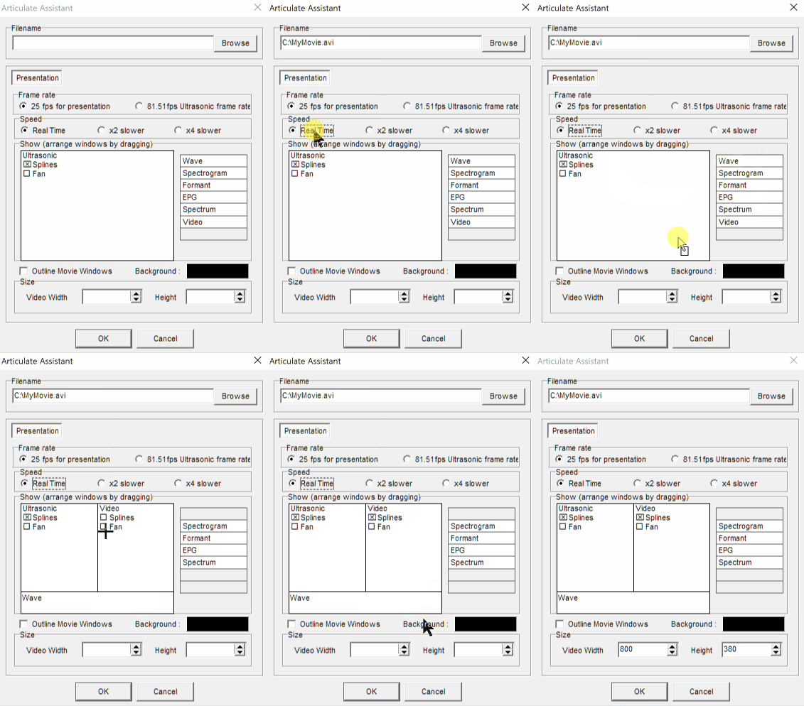
You can design a video of your data by arranging several different types of data visualisation into a layout of your choice. You can click-and-drag elements from the list on the right to arrange in the window display in the left. Each element is a visualisation of data that changes over time in your recording: in your movie, they will always be synchronized as long as your data is synchronised, and as such will be shown changing concurrently.

Click here to see how to easily synchronize data.

You can choose the location to save your movie by clicking Browse at the top-right of the dialog, or by typing a file-path at the top. You can also select playback speed, and video dimensions, and frame-rate (higher values result in smoother looking video but also much larger file-size).

The Background color is used in areas where the aspect ratio of images (eg. your recorded video) differs from the space you've given it in your chosen layout.

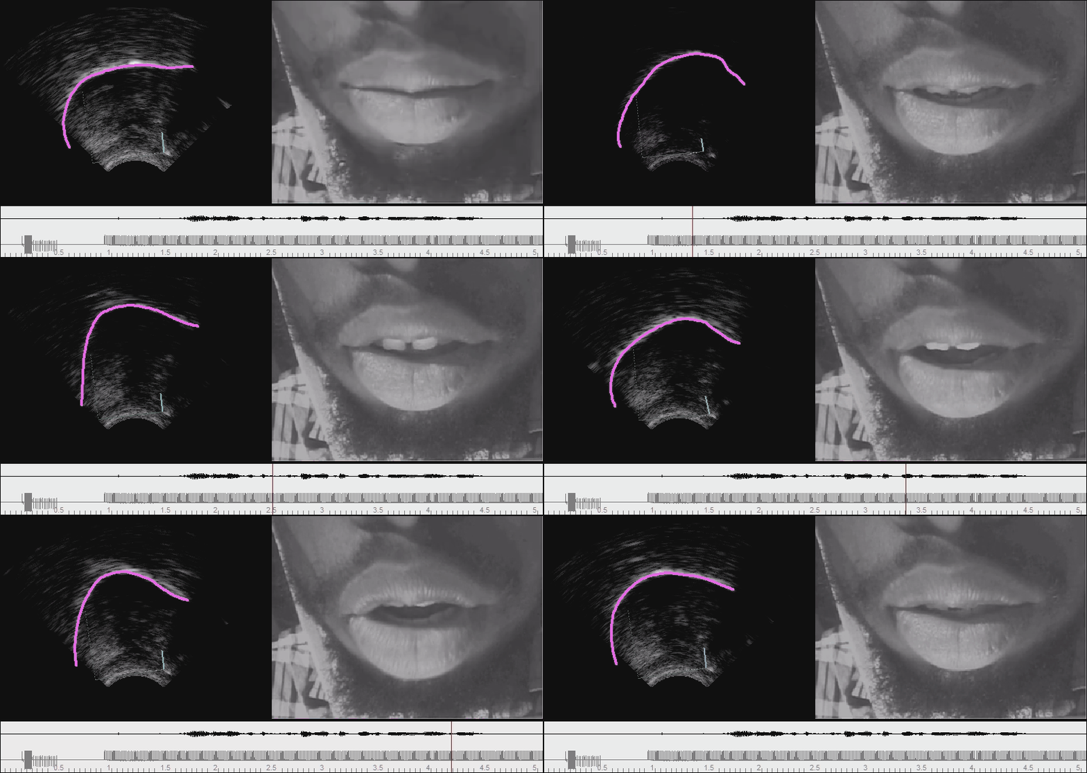
Here is an example movie made using the layout and settings shown above:

Export Data:

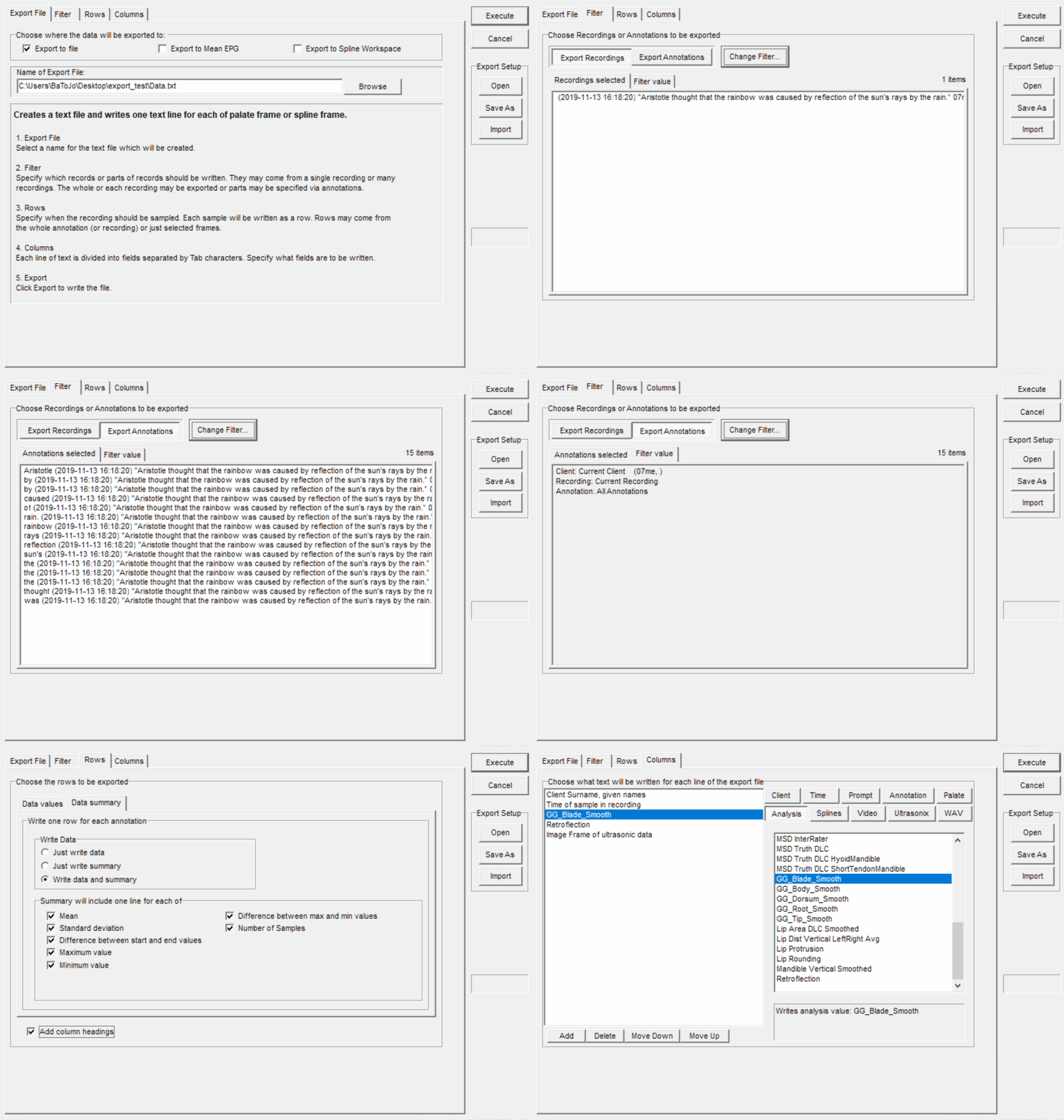
You can access this from the menu bar at the top of the screen by clicking File → Export → Data...

This dialogue creates a tab separated ascii file where each row is a time point and each column contains a data value.

The data export dialog is divided into 4 main tabs at the top. First, use the Export File tab to choose the name and location of the .csv file to create which will contain the exported data and analysis values. For .csv export, ensure that the checkbox Export to file is ticked.

Note : the Columns tab will only appear if the Export to file checkbox is ticked.

Next, go to the Filter tab: you can choose to either Export Recordings for whole recordings or Export Annotations to export only the data within the timespan of specified annotations, then click Change Filter and specify the conditions a recording or annotation must meet to be exported.

Next, in the Rows tab you must specify which time points should be included within each of the previously specified recordings or annotations. Recorded data are sampled at discrete timepoints referred to as samples or frames. In between the frame sample times, values are interpolated linearly by the software. By selecting to export every sample of your primary data type (ultrasonic, video, EPG etc) you avoid interpolated values. It is often desired to export the midpoint or N equally spaced points derived from an annotated segment. It is also possible to export the timepoint within each annotaed segment that has the maximum value of a specified variable (e.g. a distance value derived from tongue splines or palatal contact derived from EPG).

If you wanted to export a row for every frame of a particular type, you would choose All Video Frames or All Ultrasonic Frames. If you wish to export only the data from your spline-based Analysis Values, you may wish to select All Spline Keyframes to avoid data frames which have no corresponding spline or which contain interpolated values.

The Data Summary sub-tab lets you choose if you want to add some simple statistics to your exported data file. If you are planning to use tools external to AAA to analyse your data after export, it is probably better to choose Just write data.

Export Files:

You can access this from the menu bar at the top of the screen by clicking File → Export → Files...

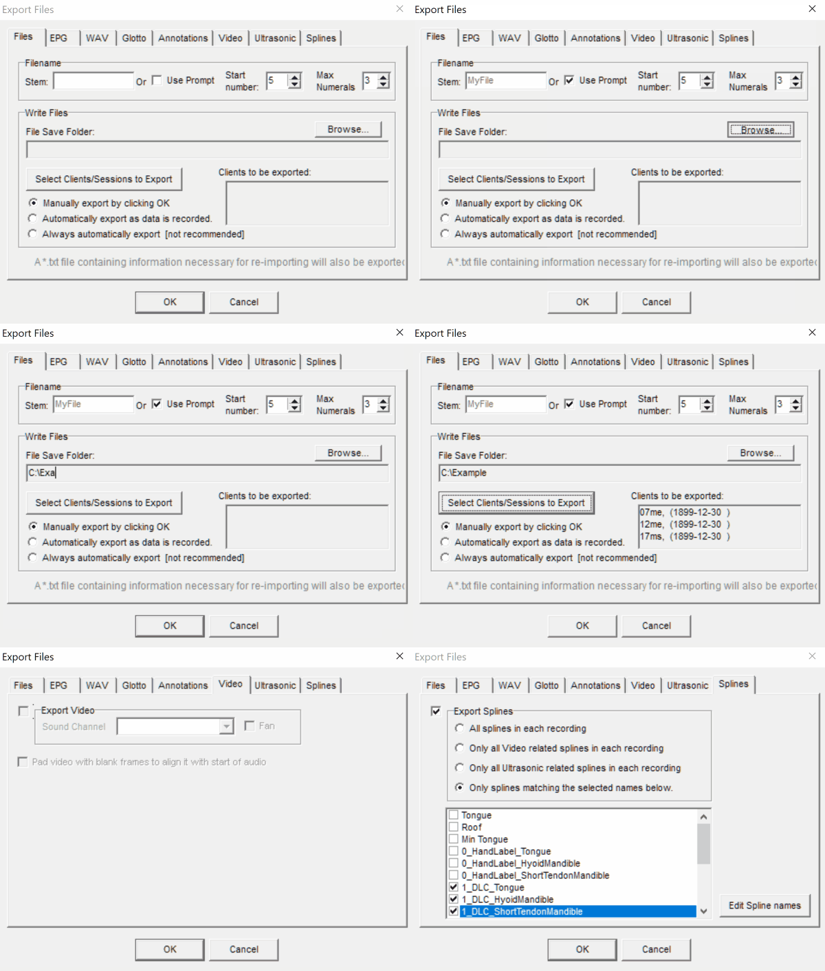
This dialog lets you choose one or more types of data stored in AAA to be saved as files on your computer in common standard file formats, making them easy to import into other software or backup. Any type of data you can record using AAA can be exported like this.

Note: This method exports the entire recording. To export only annotated regions, use the Export Data dialogue.

The tabs along the top of the dialog each correspond to a type of data, and you can visit each tab to choose whether or not to export that type of data. Each tab also has settings you can use specify data formatting, or choose a subset to export, if desired.

Files

To export, you must choose a folder as the location to save your exported data to by using the Browse button or typing in a file path. You must also click the button `Select Clients/Sessions to Export' and tick the checkboxes for every client you want to export the data for. (If you select the current client and that client has more than one recording associated with it then you can also specify a subset of those recordings to export).

For naming your exported files, you have two options:

1. You can type a file name 'stem' which will prefix all exported file names, and will automatically increment a counter for every recording exported. You can choose the number it will start at and how many digits should be used. eg. Stem File, start 1 and numerals 3 would export the first 9 files as something similar to the following:

   File001.avi
   File001.spl
   File001_Track0.wav
   File002.avi
   File002.spl
   File002_Track0.wav
   File003.avi
   File003.spl
   File003_Track0.wav
   

2. You can check the box Use Prompt to prefix each file with the full prompt text for its recording, and increment the numbers for each recording within the same prompt. If you have very long prompts this will create very long filenames. eg. Use Prompt, start 1 and numerals 3 would export the first 9 files as something similar to the following:

   Lorem ipsum001.avi
   Lorem ipsum001.spl
   Lorem ipsum001_Track0.wav
   Lorem ipsum002.avi
   Lorem ipsum002.spl
   Lorem ipsum002_Track0.wav
   Dolor sit amet001.avi
   Dolor sit amet001.spl
   Dolor sit amet001_Track0.wav
   

What order are files exported in, though? Unfortunately it's complicated. If you are exporting only one client, and have chosen a subset of sessions and recordings to export, then it will export it in the following order: For each repetition, for each prompt: export. (Where repetition here means a recording you make of the same prompt on the same client on the same day)

Thus it would be ordered like:

Prompt1-Rep1
Prompt2-Rep1
Prompt1-Rep2
Prompt2-Rep2

If, alternatively, you want to export multiple clients at once, then the order the files will be exported in will just be whatever order they were recorded in chronologically. For this reason it is advisable to check the box Use Prompt to name each exported file according to its prompt.

How does AAA manage data?

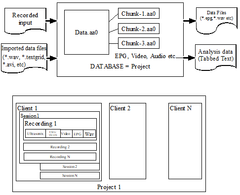
To cope with many different data streams (audio, ultrasound, video, EPG, EMA, MRI, VICON, Glottograph) recorded at different sample rates and to permit fast annotation queries and data analysis, a proprietary database forms the foundation of the software. Data can be analysed within AAA or exported in many common file formats for analysis by other software.

AAA can load any number of databases (referred to hereafter as projects), one at a time. Each project is located in a separate folder and consists of a core database file (Data.aa0) and a sequence of Chunk files (Chunk_1.aa0, Chunk_2.aa0, etc.). The Data.aa0 file contains most (but not all) of the data associated with the project. Some data such as audio, video and EPG data is too large for the computer to handle as one big file, so it is instead stored separately as Chunk files. Chunks must NOT be separated from their Data.aa0 file! The Data.aa0 file keeps a list of all the Chunk files it expects to see, so if you rename, delete or move Chunk files it will corrupt your entire project and make it unusable.

WARNING: Don't copy parts of projects! If you want to move or back-up your work, you must back-up everything in the project folder together at the same time. You must NOT modify or back-up a subset of the files in a project folder or it will corrupt your project and you won't be able to use it. When you use AAA, all the Chunk files get regularly modified and reassigned with new names. Microsoft Windows can sometimes fail to correctly show the date a Chunk file has been modified, and this can mislead people into thinking they can back up only a subset of their data.

Version-control software such as Git is a much safer and more effective way to back-up incremental changes to AAA projects, but you must always commit every change that AAA makes to the files. If you only commit a subset of changed files then you will create a corrupt commit.

Every frame or sample of data is time stamped to the nearest 100,000th of a second (10 microseconds). AAA can even cope with data that does not have a regular sample rate. The only exception to this is audio data; audio data is the ground truth for all other data streams. Audio data must have regular sample intervals and has a sample rate associated with it which is taken from the recording device. Even it this rate is inaccurate, it becomes the clock to which all the other streams are synchronised. A recording must have an audio track: other data streams cannot be recorded by AAA without audio.

The AAA software allows you to

• Create as many projects as you wish.
• Transfer data between projects.
• Import data in standard file formats. (*.wav, *.epg, PRAAT textgrid, *.avi, etc)
• Export data to standard file formats.
• Calculate values from data and export them and/or plot them.
• Create publishable quality graphics from the data.

All data within a project can be compared and analysed as a group. Each recorded data channel can be filtered, smoothed, differentiated, combined with other data channels, etc. Key features like peaks, valleys, midpoints etc can be found automatically and labelled.

Data values, durations of labelled regions and many other pieces of information can be exported to Excel or R for charting and statistical analysis. Sophisticated queries can be carried out within AAA on labelled data to extract only the information that is required.

Movies of articulatory data can be created for use in presentations and played in slow motion if required. High quality charts suitable for 600dpi journal and book publication can be generated from the various displays.

AAA provides a powerful tool for multichannel speech analysis but we are always on the lookout to improve the utility of the software. So if you have ideas for new features please get in touch and we'll see what we can do.