QCProcedures - aodn/imos-toolbox GitHub Wiki
The following automatic quality control policy and procedures are available in the Toolbox since version 2.5:
At the moment, the flag management policy is as follow :
-Any data sample in the data set is checked by the QC procedures, procedure by procedure.
-For each procedure, if a checked sample fails a test, then it gains the corresponding fail flag if the latter is higher in the flag scale than its current one. That is to say flags are overwritten when higher.
-For each procedure, all flags are first initialised to "Raw". Then, usually when the test starts they are all initialised to the relevant "fail" flag and only the "pass" test is then performed so that "pass" flags are finally provided to the successfull samples. When relevant the "fail" test is performed instead of intialising everything with "fail" flag first, so that samples which neither fail or pass the test are provided with the "Raw" flag.
-If a procedure testing a data sample uses a formula involving neighbours then the considered neighbours are the nearest ones which don't already have a flag "Bad".
-QC procedures, parameters used and results are detailed in the global attribute history. They can also be displayed in a table via the 'QC stats' button on the main panel. QC procedure details can be queried when clicking any cell from the table.
-QC parameters used are stored in a .pqc file created/updated at the same location as the input file and has the same radical name. This is so that batch re-processing can be performed with dataset specific QC parameters for each QC procedure when necessary. When a QC procedure is ran, it will try to read any existing .pqc dataset QC parameter file before the .txt generic QC parameter file. In addition, before re-running any QC set of tests, the user is asked whether to reset the different .pqc files before running the tests.
-imosHistoricalManualSetQC QC procedure reads any existing .mqc file so that any manual QC is automatically re-applied.
-Any QC test which relies on depth information takes into account the associated depth flags. If depth has been flagged not "Good", then nominal depth information is prefered to continue current QC test.
-imosTimeSeriesSpikeQC procedure uses previously defined flags in the variable state to clip/remove any bad flags already defined in the variable. The heuristic is to remove only bad flags at the beginning and towards the end of the series, so as to remove any continuous leading/trailing bad flags (e.g. from imosInOutofWaterQC).
-When exporting a NetCDF file, for each ancillary variable for QC, a variable attribute quality_control_global is automatically populated according to the ARGO reference table 2a conventions (p.57 in ARGO USER'S MANUAL - Version 2.4, March 30th 2012).
This "official IMOS standard set of procedures" and their suggested parameters will always be under ongoing development/validation so any feedback or comment is welcome.
IMOS recommends that processed data files sent to AODN data centre should only be QC'd with official IMOS standard sets of procedures. These tests are identified by the prefix "imos". Other unofficial procedures may be available for test purpose only.
These sets of QC procedures have been mainly designed to check physical variables such as temperature, salinity, velocity and pressure/depth collected either on moorings (time series) or while performing CTD profiles/casts from a boat at a specific station. Some are identified as compulsory while others are optional and should only been used when the data processor has checked that they improve the result of the QC.
In order to have consistency over processed data files and to make results easier to interpret, we recommend these tests should always been performed following the suggested order.
-
*imosImpossibleDateQC* (compulsory)
-
*imosImpossibleLocationSetQC) (compulsory)
-
*imosInOutWaterQC* (compulsory)
-
*imosGlobalRangeQC* (compulsory)
-
imosRegionalRangeQC (optional)
-
*imosImpossibleDepthQC* (compulsory)
-
imosRateOfChangeQC (optional)
-
imosStationarityQC (optional)
-
*imosSalinityFromPTQC* (compulsory)
-
*imosSideLobeVelocitySetQC* (compulsory)
-
*imosTiltVelocitySetQC* (compulsory)
-
*imosHorizontalVelocitySetQC* (compulsory)
- *imosVerticalVelocityQC* (compulsory)
-
imosSurfaceDetectionByDepthSetQC (optional)
-
imosEchoIntensitySetQC (optional)
-
imosEchoIntensityVelocitySetQC (optional)
-
*imosCorrMagVelocitySetQC* (compulsory)
-
imosPercentGoodVelocitySetQC (optional)
-
imosErrorVelocitySetQC (optional)
-
imosTier2ProfileVelocitySetQC (optional)
-
*imosHistoricalManualSetQC* (compulsory)
-
imosTimeSeriesSpikeQC (optional)
In addition to the IMOS ANMN standardised profiling CTD data post-processing procedures, IMOS recommends applying the following tests to any CTD profile data which is imported in the toolbox:
-
*imosImpossibleDateQC* (compulsory)
-
*imosImpossibleLocationSetQC* (compulsory)
-
*imosInOutWaterQC* (compulsory)
-
*imosGlobalRangeQC* (compulsory)
-
*imosImpossibleDepthQC* (compulsory)
-
imosRegionalRangeQC (optional)
-
imosVerticalSpikeQC (optional)
-
imosDensityInversionSetQC (optional)
-
*imosSalinityFromPTQC* (compulsory)
- *imosHistoricalManualSetQC* (compulsory)
The basis of most of these tests is described in Morello et al. 2011 paper, Morello et al. 2014 paper and Mantovanelli report November 2014.
Variables mentioned below are IMOS parameters code and their definition can be found in IMOS\imosParameters.txt.
Impossible date test - imosImpossibleDateQC - Compulsory
imosImpossibleDateQC checks that the TIME values are within an acceptable range. Because some instrument files contain the date information in binary format like the datenum Matlab format (decimal days from a specific date and time, where datenum('Jan-01-0000 00:00:00') returns the number 1) it is only possible to set up a generic test that only checks the full date range. Cheking the day, month, hour, minute or second values separately (minimum/maximum valid values for minutes, months, days in February, etc...) is not possible in our case.
| Parameter checked | Pass test flag | Fail test flag |
|---|---|---|
| TIME | 1-Good data | 4-Bad data |
The samples that pass the test are the one verifying TIME >= dateMin and TIME <= dateMax.
An imosImpossibleDateQC.txt parameter file allows the user to define the dateMin and dateMax values. See default configuration below :
dateMin = 01/01/2007

dateMax =
By default, if dateMax is left empty then dateMax is the current date at the time of test.
Since this test is critical, a warning message is displayed if some samples fail the test and an error message is raised when all points fail the test.
Impossible location test - imosImpossibleLocationSetQC - Compulsory
imosImpossibleLocationSetQC checks the LATITUDE and LONGITUDE values against a nominal position and acceptable range for the relevant mooring site. Useful to detect typos in positions documented in the metadata/deployment database.
| Parameters checked | Pass test flag | Fail test flag |
|---|---|---|
| LONGITUDE, LATITUDE | 1-Good data | 3-Bad data that are potentially correctable |
The site name is retrieved from the deployment database in the field Site of the table DeploymentData and then IMOS sites information and parameters are read from IMOS\imosSites.txt for the relevant site. See example of default parameter file below :
% Definitions and descriptions of IMOS moorings/stations sites.

%

% These information are used in impossible location QC test.

% distanceKmPlusMinusThreshold overrules other thresholds.

%

% Format:

%

% name, nominalLongitude, nominalLatitude, longitudePlusMinusThreshold, latitudePlusMinusThreshold, distanceKmPlusMinusThreshold

%

NRSMAI, 	148.2333, 		-42.59667, 		0.025, 	0.025, 	2.5

NRSNSI, 	153.58, 		-27.389, 		0.025, 	0.025, 	2.5

...
The impossible location test can be performed according to 2 variations:
- distanceKmPlusMinusThreshold is not Nan (default case):
The LONGITUDE and LATITUDE samples values that pass the test are the one verifyingdistance between coordinates (LONGITUDE, LATITUDE) and (nominalLongitude, nominalLatitude) <= distanceKmPlusMinusThreshold.
In this case, positions are expected to be in a circle centered on the nominal position and which radius is distanceKmPlusMinusThreshold. LATITUDE and LONGITUDE are checked together as a position and gain the same flag.
- distanceKmPlusMinusThreshold is Nan :
The LONGITUDE samples values that pass the test are the one verifyingLONGITUDE >= nominalLongitude - longitudePlusMinusThresholdandLONGITUDE <= nominalLongitude + longitudePlusMinusThreshold.
The LATITUDE samples values that pass the test are the one verifyingLATITUDE >= nominalLatitude - latitudePlusMinusThresholdandLATITUDE <= nominalLatitude + latitudePlusMinusThreshold.
In this case, positions are expected to be in a square centered on the nominal position and which width is 2longitudePlusMinusThreshold and height 2latitudePlusMinusThreshold. LATITUDE and LONGITUDE are checked separately and gain their own flag.
Since this test is critical and can easily be corrected, an error message is triggered if some samples fail the test.
In/Out water test - imosInOutWaterQC - Compulsory
imosInOutWaterQC flags any variable sample which TIME values are not between the first and last time when the instrument is actually in position collecting data for time series purpose. Between these two times, data is deliberately left non QC'd.
| Parameters checked | Pass test flag | Fail test flag |
|---|---|---|
| Any variable | 0-No QC performed | 4-Bad data |
The samples that pass the test are the ones which TIME values are verifying TIME >= in water time and TIME <= out water time.
in water time can be one of these date information taken from fields of the table DeploymentData in the deployment database, in this order of preference :
- TimeFirstGoodData : Time of first good data.
- TimeFirstInPos : Time instrument first in position.
- TimeFirstWet : Time instrument first in water.
- TimeSwitchOn : Time instrument is switched on.
out water time can be one of these date information taken from fields of the table DeploymentData in the deployment database, in this order of preference :
- TimeLastGoodData : Time of last good data.
- TimeLastInPos : Time instrument last in position.
- TimeOnDeck : Time instrument on deck.
- TimeSwitchOff : Time instrument is switched off.
imosInOutWaterQC test raises an error if time values are significantly out against the deployment database station times. In that case, the data processor needs to check and correct one or the other.
Global range test - imosGlobalRangeQC - Compulsory
imosGlobalRangeQC checks that the parameter's values are within a global valid range. The default list of parameters impacted by this test is found in AutomaticQC\imosGlobalRangeQC.txt.
| Parameters checked | Pass test flag | Fail test flag |
|---|---|---|
| TEMP, PSAL, PRES, PRES_REL, DEPTH, CPHL, CHLU, CHLF, DOXY, DOX1, DOX2, UCUR, VCUR, WCUR, CDIR, CSPD | 1-Good data | 4-Bad data |
The samples that pass the test are the ones which parameter's values are verifying PARAMETER >= validMin and PARAMETER <= validMax.
The IMOS\imosParameters.txt file contains validMin and validMax values for each IMOS parameters. The validMin and validMax values of the impacted parameters by this test have been set based on suggested values from the following documents : Argo quality control manual - Version 2.7, 3 January 2012 and EuroGOOS Recommendations for in-situ data Near Real Time Quality Control - Version 1.2, December 2010.
See below default list of impacted parameters by this test and their validMin / validMax values from imosParameters.txt file :
%

% A list of all IMOS compliant parameter names, associated standard names from version 20

% (http://cf-pcmdi.llnl.gov/documents/cf-standard-names/standard-name-table/20/cf-standard-name-table.html/),

% units of measurement, fill values, and valid min/max values. This list has been copied

% verbatim from the IMOS NetCDF User's manual version 1.3, and the IMOS NetCDF

% File Naming Convention version 1.3. Entries are in the following format:

%

%   parameter name, is cf parameter, standard/long name, units of measurement, data code, fillValue, validMin, validMax, NetCDF 3.6.0 type

%

% For parameters which are specified as a percentage, use the word 'percent'

% in this file - this will be automatically converted into a '%' sign. This is

% necessary because Matlab will interpret literal '%' signs as the beginining

% of a comment.

%


CDIR,     1, direction_of_sea_water_velocity,                               Degrees clockwise from true North, V, 999999.0, 0.0,     360.0,    float

CPHL,     1, mass_concentration_of_chlorophyll_in_sea_water,                mg m-3,                            K, 999999.0, 0.0,     100.0,    float

CHLF,     1, mass_concentration_of_chlorophyll_in_sea_water,                mg m-3,                            K, 999999.0, 0.0,     100.0,    float

CHLU,     1, mass_concentration_of_chlorophyll_in_sea_water,                mg m-3,                            K, 999999.0, 0.0,     100.0,    float

CSPD,     1, sea_water_speed,                                               m s-1,                             V, 999999.0, 0.0,     10.0,     float

DEPTH,    1, depth,                                                         m,                                 Z, 999999.0, -5.0,    12000.0,  float

DOXY,     1, mass_concentration_of_oxygen_in_sea_water,                     kg m-3,                            O, 999999.0, 0.0,     29.0,     float

DOX1,     1, mole_concentration_of_dissolved_molecular_oxygen_in_sea_water, umol l-1,                          O, 999999.0, 0.0,     900000.0, float

DOX2,     1, moles_of_oxygen_per_unit_mass_in_sea_water,                    umol kg-1,                         O, 999999.0, 0.0,     880000.0, float

PRES,     1, sea_water_pressure,                                            dbar,                              Z, 999999.0, -5.0,    12000.0,  float

PRES_REL, 1, sea_water_pressure_due_to_sea_water,                           dbar,                              Z, 999999.0, -15.0,   12000.0,  float

PSAL,     1, sea_water_salinity,                                            psu,                               S, 999999.0, 2.0,     41.0,     float

TEMP,     1, sea_water_temperature,                                         Celsius,                           T, 999999.0, -2.5,    40.0,     float

UCUR,     1, eastward_sea_water_velocity,                                   m s-1,                             V, 999999.0, -10.0,   10.0,     float

VCUR,     1, northward_sea_water_velocity,                                  m s-1,                             V, 999999.0, -10.0,   10.0,     float

WCUR,     1, upward_sea_water_velocity,                                     m s-1,                             V, 999999.0, -5.0,    5.0,      float
If valid ranges are not documented for a parameter or are of same value for Min and Max then the test is not performed.
Regional range test - imosRegionalRangeQC - Optional
imosRegionalRangeQC checks that the variables values are within a regional range which is site specific. This test is available at one's discretion who is fully aware of the regional ranges applied to his datasets. The default list of sites and variables impacted by this test is found below.
| Sites and variables checked | Pass test flag | Fail test flag |
|---|---|---|
| See AutomaticQC/imosRegionalRangeQC.txt | 1-Good data | 4-Bad data |
The samples that pass the test are the ones which parameters values are verifying PARAMETER >= regionalRangeMin and PARAMETER <= regionalRangeMax.
Regional ranges are specified for each site and parameter in the AutomaticQC/imosRegionalRangeQC.txt parameter file.
See example of default parameter file below :
% Definitions and descriptions of IMOS moorings/stations sites regional ranges.

%

% These information are used in the regional range QC test.

% These thresholds values were taken from an histogram distribution

% analysis either from historical water samples or in-situ sensor data

%

% Format:

%

% siteName, IMOSParameter, regionalRangeMin, regionalRangeMax

%

NRSNSI, PSAL, 31.3, 38.7

NRSNSI, TEMP, 9, 33

NRSMAI, PSAL, 27.5, 38.9

NRSMAI, TEMP, 5, 25

...
If regional ranges are not documented for a site and parameter, or are of same value for Min and Max then the test is not performed.
The test is not performed and a warning message is displayed if the current processed site is not documented in the parameter file.
Impossible depth test - imosImpossibleDepthQC - Compulsory
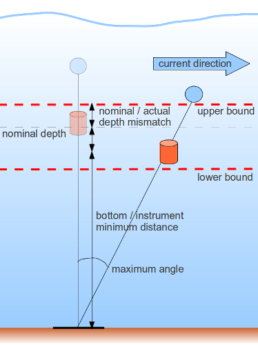
imosImpossibleDepthQC checks that the pressure/depth data are given within an acceptable range. Basically, the test checks that the instrument is close to its nominal depth, allowing enough flexibility to cope with possible mismatch between nominal and actual depth when deployed, and knock down events related to strong current events.
| Parameters checked | Pass test flag | Fail test flag |
|---|---|---|
| PRES, PRES_REL, DEPTH | 1-Good data | 4-Bad data |
The samples that pass the test are the ones which depth values are verifying DEPTH >= lower bound and DEPTH <= upper bound:
-
upper bound = instrument nominal depth - allowed maximum mismatch between nominal and actual depth lower bound = instrument nominal depth + allowed maximum mismatch between nominal and actual depth + allowed minimum distance between site nominal depth and instrument depth * (1 - cos(allowed maximum knock down angle)
Indeed, a greater range should be allowed for instruments close to the surface and which site is deep (during strong current events an instrument on a mooring is more likely to drop than rise from its nominal depth), with :
minimum distance between site nominal depth and instrument depth = site nominal depth - (instrument nominal depth + allowed maximum mismatch between nominal and actual depth)
The allowed maximum mismatch between nominal and actual depth and allowed maximum knock down angle values can be modified in the imosImpossibleDepth.txt parameter file. Default values have been set respectively to 15m and 70deg. These values are based on experience should be updated if greater values are experienced.
Finally, the resulting possible depth range cannot be out of the water or deeper than the relevant site nominal depth + allowed maximum mismatch between nominal and actual depth.
If the site nominal depth is not documented, then the site depth at deployment is used.
If the instrument nominal depth is not documented, then the instrument nominal height and site nominal depth (or site depth at deployment) are used.
The test is not performed and a warning is diplayed if there is not enough nominal depth/height information provided.
imosImpossibleDepthQC checks that the depth/pressure values are between 0 and BOT_DEPTH + 20%. If dealing with a dimension an error message is raised (CTD processing and/or site_nominal_depth / site_depth_at_station need to be checked), otherwise the usual flagging is performed.
Vertical spike test - imosVerticalSpikeQC - Optional
imosVerticalSpikeQC is looking for spikes among vertically adjacent triplet of samples. This test is for profile mode only and is available at one's discretion who is fully aware of the algorithm and flags used.
| Parameters checked | Pass test flag | Fail test flag |
|---|---|---|
| TEMP, PSAL, PRES, PRES_REL, DEPTH, CPHL, CHLU, CHLF, DOXY, DOX1, DOX2 | 1-Good data | 3-Bad data that are potentially correctable |
The algorithm used here is the same used by the Australian National Mooring Facility Ocean Gliders (ANFOG) and ARGO's spike test.
The samples that pass the test are the ones with parameter's value Vn verifying the test |Vn - (Vn+1 + Vn-1)/2| - |(Vn+1 - Vn-1)/2| <= threshold.
The provided failing flag is deliberately set to 3 (Bad data that are potentially correctable). This kind of test cannot be right in any case so we want to use another flag than the 4 (Bad data) to attract the user's attention on specific areas in the profile that need a closer look and investigation before use.
An imosVerticalSpikeQC.txt parameter file allows the user to define the threshold values to use. See default parameter file below :
TEMP = 6

PSAL = 0.9

PRES = 3

PRES_REL = 3

DEPTH = 3

CPHL = PABIM

CHLU = PABIM

CHLF = PABIM

DOXY = PABIM

DOX1 = PABIM

DOX2 = PABIM
PABIM is equivalent to the following formula :
|median(Vn-2,Vn-1,Vn,Vn+1,Vn+2)| + |standard_deviation(Vn-2,Vn-1,Vn,Vn+1,Vn+2)|
Threshold values have been set based on suggested values from the following documents : Argo quality control manual - Version 2.7, 3 January 2012, EuroGOOS Recommendations for in-situ data Near Real Time Quality Control - Version 1.2, December 2010 and PABIM White Book on Oceanic Autonomous Platforms for Biogchemical Studies: Instrumentation and Measure - Version 1.3, February 2010.
Density inversion test - imosDensityInversionSetQC - Optional
imosDensityInversionSetQC flags bad any PSAL + TEMP + CNDC + DENS value that shows an inversion in density or an increase/decrease in density that is greater than a threshold set in imosDensityInversionSetQC.txt.This test is for profile mode only and is available at one's discretion who is fully aware of the algorithm and flags used.
| Parameters checked | Pass test flag | Fail test flag |
|---|---|---|
| TEMP, PSAL, CNDC, DENS | 1-Good data | 4-Bad data |
The algorithm used here is the same used by Argo Quality Control manual v2.7:
This test compares potential density between valid measurements in a profile, in both
directions, i.e. from top to bottom, and from bottom to top. Values of temperature and
salinity at the same pressure level P i should be used to compute potential density ρ i (or σ i
= ρ i − 1000) kg m −3 , referenced to the mid-point between P i and the next valid pressure
level P i+1 . A threshold of 0.03 kg m −3 should be allowed for small density inversions.
Action: From top to bottom, if the potential density calculated at the greater pressure is
less than that calculated at the lesser pressure by more than 0.03 kg m −3 , both the
temperature and salinity values should be flagged as bad data. From bottom to top, if the
potential density calculated at the lesser pressure is greater than that calculated at the
greater pressure by more than 0.03 kg m −3 , both the temperature and salinity values
should be flagged as bad data. Bad temperature and salinity values should be removed
from the TESAC distributed on the GTS.
.
An imosDensityInversionSetQC.txt parameter file allows the user to define the threshold values to use. See default parameter file below :
threshold = 0.03Rate of change test - imosRateOfChangeQC - Optional
imosRateOfChangeQC is looking for important changes in values among temporally adjacent triplet (or pair) of samples. This test is mostly useful for time series data and is available at one's discretion who is fully aware of the algorithm and flags used.
| Parameters checked | Pass test flag | Fail test flag |
|---|---|---|
| TEMP, PSAL, PRES, PRES_REL, DEPTH, CPHL, CHLU, CHLF, DOXY, DOX1, DOX2, UCUR, VCUR, WCUR, CSPD | 1-Good data | 3-Bad data that are potentially correctable |
The samples that pass the test are the ones with parameter's value Vn verifying the test |Vn - Vn-1| + |Vn - Vn+1| <= 2*(threshold).
If the previous (or following) sample is missing then the test becomes |Vn - Vn-1| <= 1*(threshold) (respectively |Vn - Vn+1| <= 1*(threshold)).
It is only considering adjacent samples with flags lower or equal to 3 (Bad data that are potentially correctable). If the test involves consecutive samples with a time period greater than 1h between them then the test is cancelled for this triplet or pair.
The provided failing flag is deliberately set to 3 (Bad data that are potentially correctable). This kind of test cannot be right in any case so we want to use another flag than the 4 (Bad data) to attract the user's attention on specific areas in the time series that need a closer look and investigation before use.
An imosRateOfChangeQC.txt parameter file allows the user to define the threshold values to use. See default parameter file below :
TEMP = 2*stdDev

PSAL = 2*stdDev

PRES = 2*stdDev

PRES_REL = 2*stdDev

DEPTH = 2*stdDev

CPHL = 2*stdDev

CHLU = 2*stdDev

CHLF = 2*stdDev

DOXY = 2*stdDev

DOX1 = 2*stdDev

DOX2 = 2*stdDev

UCUR = 2*stdDev

VCUR = 2*stdDev

WCUR = 2*stdDev

CSPD = 2*stdDev
Threshold values have been set based on suggested values from the following document : Argo quality control manual - Version 2.7, 3 January 2012 and EuroGOOS Recommendations for in-situ data Near Real Time Quality Control - Version 1.2, December 2010.
By default, the gradient is compared to 2 times the standard deviation observed on the first month of 'Good' data so far (which means taking into account only the data with flags lower or equal to 2 (Probably good) that have been provided by previously performed QC tests).
Stationarity test - imosStationarityQC - Optional
imosStationarityQC checks that consecutive equal values of a parameter don't exceed a maximum number. This test is available at one's discretion who is fully aware of the algorithm and flags used.
The algorithm used is based on the stationarity test from IOC. The default list of parameters impacted by this test is found in imosGlobalRangeQC.txt.
| Parameters checked | Pass test flag | Fail test flag |
|---|---|---|
| TEMP, PSAL, PRES, PRES_REL, DEPTH, CPHL, CHLU, CHLF, DOX1, DOX2, UCUR, VCUR, WCUR, CDIR, CSPD | 1-Good data | 4-Bad data |
The samples with consecutive equal values that pass the test are the ones verifying the test number of consecutive points <= 24*(60/delta_t) with delta_t the sampling interval in minutes.
It is only considering adjacent samples with flags lower or equal to 3 (Bad data that are potentially correctable).
Flag inheritance test on Salinity - imosSalinityFromPTQC - Compulsory
imosSalinityFromPTQC checks that any salinity measurement has its flag equals or greater than any pressure/depth, conductivity and temperature measurements on the same sample. If not, it gives the highest observed flag. When depth exists, pressure flags are not taken into accountso that re-calculated "good" depth from nearby P sensor has priority over a failing pressure.
| Parameters checked | Pass test flag | Fail test flag |
|---|---|---|
| PSAL | 1-Good data | highest flag from temperature, depth and pressure measurements of the same sample |
ADCP side lobe contamination test - imosSideLobeVelocitySetQC - Compulsory
imosSideLobeVelocitySetQC finds for each timestamp what is the HEIGHT_ABOVE_SENSOR from which any data sample is contaminated by side lobes effect (close to the surface or bottom). Impacted data samples are then flagged accordingly. This test can be applied on any ADCP data providing we know the beam angle of the ADCP transducer. It is based on Nortek's documentation.
In the case of upward looking ADCPs, the measured depth at the instrument is the distance to surface, while with downward looking ones the distance to surface is global attribute site_nominal_depth or site_depth_at_deployment - measured depth at the instrument.
| Parameters checked | Pass test flag | Fail test flag |
|---|---|---|
| UCUR, VCUR, WCUR, CSPD, CDIR | 1-Good data | 4-Bad data |
The samples that pass the test are the ones with HEIGHT_ABOVE_SENSOR values verifying depth of bin > contaminated depth with contaminated depth = instrument depth - (instrument depth * cos(beam angle) - 1/2 * bin size). The following figure illustrates the case of an ADCP set on the sea bottom :
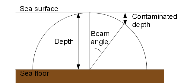
Subtracting 1/2 of the size of a bin to the non-contaminated height enables us to be conservative in order to make sure that the data in the first bin below the contaminated depth hasn't been computed from any contaminated signal.
ADCP tilt test - imosTiltVelocitySetQC - Compulsory
imosTiltVelocitySetQC is a two-level test which flags velocity data depending on the tilt values. Most ADCPs see their performance degraded with increasing tilt.
For RDI ADCPs, compass measurements are affected and fail to meet specifications when a first tilt threshold is exceeded. When the second threshold is exceeded coordinates transform and bin-mapping operations are also affected.
For Nortek ADCPs, velocity data accuracy fails to meet specifications when the first tilt threshold is exceeded. When the second is exceeded then velocity data becomes unreliable.
| Parameters checked | Pass test flag | Fail test flag |
|---|---|---|
| UCUR, VCUR, WCUR, CSPD, CDIR | 1-Good data | two-level flag |
For each sample, the tilt is computed using the following formula : TILT = acos(sqrt(1 - sin(ROLL)^2 - sin(PITCH)^2))
A whole profile is then flagged with the relevant flag any time the tilt is greater than one of the two identified thresholds.
Default thresholds have been identified based on RDI and Nortek documentation as well as on communications with RDI technicians, and are stored in imosTiltVelocitySetQC.txt for the following instruments :
| Make/Model | First tilt treshold | Second tilt Threshold | First flag | Second flag |
|---|---|---|---|---|
| sentinel | 15 | 22 | 2 Probably_good_data | 3 Bad_data_that_are_potentially_correctable |
| monitor | 15 | 22 | 2 Probably_good_data | 3 Bad_data_that_are_potentially_correctable |
| longranger | 15 | 50 | 2 Probably_good_data | 3 Bad_data_that_are_potentially_correctable |
| long ranger | 15 | 50 | 2 Probably_good_data | 3 Bad_data_that_are_potentially_correctable |
| quartermaster | 15 | 50 | 2 Probably_good_data | 3 Bad_data_that_are_potentially_correctable |
| nortek | 20 | 30 | 2 Probably_good_data | 3 Bad_data_that_are_potentially_correctable |
Horizontal velocity test - imosHorizontalVelocitySetQC - Compulsory
imosHorizontalVelocitySetQC checks horizontal velocity values against a maximum threshold.
| Parameters checked | Pass test flag | Fail test flag |
|---|---|---|
| UCUR, VCUR, CSPD | 1-Good data | 4-Bad data |
Samples that pass the test are the ones verifying |UCUR + i*VCUR| <= hvel.
With hvel default value of 2.0m.s-1 stored in imosHorizontalVelocitySetQC.txt.
This test is part of a procedure implemented by the U.S. National Data Buoy Center, MI, and detailed in Crout et al. (2005).
This same methodology has been applied for the Quality Control of the mooring data collected during the INSTANT (International Nusantara STratification ANd Transport program) deployments in the outflow straits - Lombok Strait and Timor Passage. In addition, the determination of the parameters used in this methodology has been described by Janet Sprintall (2007) in this document (see Appendix 2). Its result specified the default parameters values used in the QC procedure.
Surface Detection By Depth Test - imosSurfaceDetectionByDepthSetQC - Optional
This test detects the bottom or sea surface based on the deployment metadata and the beam length, by comparing the beam length of the ADCP, the instrument depth, and site depth. The marking is based on simple length comparison against the "visible water column" at a given time for the adcp instrument. Both upward/downward looking instruments are supported. See also IMOS.adcp.bin_in_water.
Vertical velocity test - imosVerticalVelocityQC - Compulsory
imosVerticalVelocityQC checks vertical velocity values against a maximum threshold.
| Parameters checked | Pass test flag | Fail test flag |
|---|---|---|
| WCUR | 1-Good data | 4-Bad data |
Samples that pass the test are the ones verifying |WCUR| <= vvel.
With vvel default value of 0.2m.s-1 stored in imosVerticalVelocityQC.txt.
This test is part of a procedure implemented by the U.S. National Data Buoy Center, MI, and detailed in Crout et al. (2005).
This same methodology has been applied for the Quality Control of the mooring data collected during the INSTANT (International Nusantara STratification ANd Transport program) deployments in the outflow straits - Lombok Strait and Timor Passage. In addition, the determination of the parameters used in this methodology has been described by Janet Sprintall (2007) in this document (see Appendix 2). Its result specified the default parameters values used in the QC procedure.
ADCP echo intensity test - imosEchoIntensitySetQC - Optional
imosEchoIntensitySetQC looks at the difference in echo intensity between adjacent vertical bins. When this difference is greater than a certain threshold, the bin is marked as bad.
The test is more flexible than the original EchoIntensityVelocitySetQC (see below), in the sense that the test can be executed only from a pre-defined bin-number - bound_by_index (e.g. mark only from bin number=10), be clipped to depth levels - bound_by_depth (mark only above/below =100m), and if we should expand/propagate a bad bin flag to other bins further away from the instrument - propagate flag.
This test is available at one's discretion who is fully aware of the algorithm and demands expertise to set relevant thresholds for each dataset.
ADCP echo intensity test - imosEchoIntensityVelocitySetQC - Optional
imosEchoIntensityVelocitySetQC looks at the difference in echo intensity between adjacent vertical bins. When this difference is greater than a certain threshold for at least 3 beams, this means an obstacle (surface or bottom) is detected and from there, any further bin is flagged bad. This test is also available at ones discretion who is fully aware of the algorithm and demands expertise to set relevant thresholds for each dataset.
This test raises a warning if applied without ABSICn being vertically bin-mapped.
| Parameters checked | Pass test flag | Fail test flag |
|---|---|---|
| UCUR, VCUR, WCUR, CSPD, CDIR | 1-Good data | 4-Bad data |
-
ABSICn(current bin)-ABSICn(previous bin) <= ea_thresh(performed on the 4 beams, we look at the difference in amplitude between vertically consecutive pair of bins. At least 3 beams differences must be less than ea_thresh in order to pass the test. When a bin is flagged bad, then all the bins further it are flagged bad as well.).
With ea_thresh default value of 30 counts suggested by Janet Sprintall for the RDI Workhorse Quartermaster ADCP 300kHz. However relevant threshold value needs to be set for each dataset! It is stored in imosEchoIntensityVelocitySetQC.txt.
This test is part of a procedure implemented by the U.S. National Data Buoy Center, MI, and detailed in Crout et al. (2005).
This same methodology has been applied for the Quality Control of the mooring data collected during the INSTANT (International Nusantara STratification ANd Transport program) deployments in the outflow straits - Lombok Strait and Timor Passage. In addition, the determination of the parameters used in this methodology has been described by Janet Sprintall (2007) in this document (see Appendix 2). Its result specified the default parameters values used in the QC procedure.
ADCP correlation magnitude test - imosCorrMagVelocitySetQC - Compulsory
imosCorrMagVelocitySetQC test checks that there is sufficient signal to noise ratio to obtain good quality data via the measure of a pulse-to-pulse correlation in a ping. At each bin, if at least 2 beams see their correlation value greater than a threshold value then the sample at that bin passes the test.
This test raises a warning if applied without CMAGn being vertically bin-mapped.
| Parameters checked | Pass test flag | Fail test flag |
|---|---|---|
| UCUR, VCUR, WCUR, CSPD, CDIR | 1-Good data | 4-Bad data |
-
CMAGn > cmag(performed on the 4 beams, at least 2 must be greater than cmag in order to pass to the test)
With cmag default value of 64 suggested by Alessandra Mantovanelli's report. However, relevant threshold value might need to be set for each dataset. It is stored in imosCorrMagVelocitySetQC.txt.
This test is part of a procedure implemented by the U.S. National Data Buoy Center, MI, and detailed in Crout et al. (2005).
This same methodology has been applied for the Quality Control of the mooring data collected during the INSTANT (International Nusantara STratification ANd Transport program) deployments in the outflow straits - Lombok Strait and Timor Passage. In addition, the determination of the parameters used in this methodology has been described by Janet Sprintall (2007) in this document (see Appendix 2). Its result specified the default parameters values used in the QC procedure.
ADCP percent good test - imosPercentGoodVelocitySetQC - Optional
imosPercentGoodVelocitySetQC test checks that the percentage of good 3 beams and 4 beams solutions is greater than a certain threshold. A percentage of bad solution is based on low correlation and fish detection. This test is available at ones discretion who is fully aware of the algorithm and demands expertise to set relevant thresholds for each dataset.
| Parameters checked | Pass test flag | Fail test flag |
|---|---|---|
| UCUR, VCUR, WCUR, CSPD, CDIR | 1-Good data | 4-Bad data |
-
PERG1 + PERG4 > pgood(performed on the 1st and 4th value only: represents the percentage good of 3 and 4 beam solutions in earth coordinates configuration)
With pgood default value of 50% suggested Janet Sprintall for the RDI Workhorse Quartermaster ADCP 300kHz. However relevant threshold value needs to be set for each dataset! It is stored in imosPercentGoodVelocitySetQC.txt.
This test is part of a procedure implemented by the U.S. National Data Buoy Center, MI, and detailed in Crout et al. (2005). Thanks to Rebecca Cowley (CSIRO Hobart) this procedure has been corrected from a mis-interpretation, putting more faith into the original document from RDI Darryl R Symonds (2006).
This same methodology has been applied for the Quality Control of the mooring data collected during the INSTANT (International Nusantara STratification ANd Transport program) deployments in the outflow straits - Lombok Strait and Timor Passage. In addition, the determination of the parameters used in this methodology has been described by Janet Sprintall (2007) in this document (see Appendix 2). Its result specified the default parameters values used in the QC procedure.
ADCP error velocity test - imosErrorVelocitySetQC - Optional
imosErrorVelocitySetQC test checks that the horizontal error velocity (difference between two independent estimates, basically two pair of beams) is smaller than a certain threshold so that the assumption of horizontal flow homogeneity is reasonable. This test is only available in 4 beams solution and shouldn't flag as bad any 3 beam solution. This test is available at ones discretion who is fully aware of the algorithm and demands expertise to set relevant thresholds for each dataset.
| Parameters checked | Pass test flag | Fail test flag |
|---|---|---|
| UCUR, VCUR, WCUR, CSPD, CDIR | 1-Good data or 2-Probably good data if ECUR is NaN | 4-Bad data |
- Good data if:
ECUR >= ervm - err_vel & ECUR <= ervm + err_vel; - NaNs means 3 beam solution only and should not fail this test but gain a probably good flag instead
With:
ervm the ECUR mean, this is to account for the fact that the error velocity is very rarely centered around zero. err_vel default value of 0.15m.s-1 suggested Janet Sprintall for the RDI Workhorse Quartermaster ADCP 300kHz. However relevant threshold value needs to be set for each dataset! It is stored in imosErrorVelocitySetQC.txt.This same methodology has been applied for the Quality Control of the mooring data collected during the INSTANT (International Nusantara STratification ANd Transport program) deployments in the outflow straits - Lombok Strait and Timor Passage. In addition, the determination of the parameters used in this methodology has been described by Janet Sprintall (2007) in this document (see Appendix 2). Its result specified the default parameters values used in the QC procedure.
ADCP tier 2 profile test - imosTier2ProfileVelocitySetQC - Optional
imosTier2ProfileVelocitySetQC test checks that more than 50% of the bins in the water column (imosEchoIntensityVelocitySetQC test gives where the surface/bottom starts) in a profile have passed all of the 5 other velocity tests otherwise the entire profile fails. This test is available at ones discretion who is fully aware of the algorithm and demands expertise to set relevant thresholds for each dataset.
| Parameters checked | Pass test flag | Fail test flag |
|---|---|---|
| UCUR, VCUR, WCUR, CSPD, CDIR | 1-Good data | 4-Bad data |
The bin samples that pass the test are the ones passing the 5 sub-tests and which belong to a profile which has less than 50% of its bins failing the 5 sub-tests :
- imosHorizontalVelocitySetQC
- imosVerticalVelocityQC
- imosErrorVelocitySetQC
- imosPercentGoodVelocitySetQC
- imosCorrMagVelocitySetQC
This test is part of a procedure implemented by the U.S. National Data Buoy Center, MI, and detailed in Crout et al. (2005). Thanks to Rebecca Cowley (CSIRO Hobart) this procedure has been corrected from a mis-interpretation, putting more faith into the original document from RDI Darryl R Symonds (2006).
Historical manual QC test - imosHistoricalManualSetQC - Compulsory
Anytime a manual QC is performed, a .mqc file is created/updated with a new information about what has been flagged where and with with which flag and comment. The file is at the same location as the input file and has the same radical name.
imosHistoricalManualSetQC QC procedure reads any existing .mqc file so that any manual QC is automatically re-applied.
These QC procedures are still under development/validation and should only be used with full knowledge for test purpose. IMOS do not recommend these tests to be performed on data files that will be sent to AODN data centre.
Climatology range test - climatologyRangeQC
climatologyRangeQC checks parameter's values against a climatology. In order to perform this test, you need a climatology file for each of your mooring site. In your toolboxProperties.txt configuration file, make sure the directory where lay those climatology files is documented :
% default directory for climatology data

importManager.climDir = E:\Documents and Settings\ggalibert\My Documents\IMOS_toolbox\data_files_examples\CLIMATOLOGIES\
Examples of climatology files and documents detailing the methodology applied to create them can be found here.
| Parameters checked | Pass test flag | Fail test flag |
|---|---|---|
| Any parameter found in the climatology file | 1-Good data | 3-Bad data that are potentially correctable |
The samples that pass the test are the ones which parameters values are verifying PARAMETER >= climatologyRangeMin and PARAMETER <= climatologyRangeMax.
Climatology ranges are specified in a generic way in the AutomaticQC/climatologyRangeQC.txt parameter file.
See example of default parameter file below :
rangeMin = min(mean - 6*stdDev, mini-2*stdDev)

rangeMax = max(mean + 6*stdDev, maxi+2*stdDev)
Parameters mean, stdDev, mini and maxi are respectively the mean, standard deviation, minimum value and maximum value from a temporal bin at a specific depth, found in the relevant climatology file. For each data sample, the relevant parameters are extracted so that they fall within the proper temporal bin and the climatology depth is the nearest from the actual depth of the sample.
The provided failing flag is deliberately set to 3 (Bad data that are potentially correctable). This kind of test cannot be right in any case so we want to use another flag than the 4 (Bad data) to attract the user's attention on specific areas in the time series that need a closer look and investigation before use.
If the site information is not documented in the metadata, the data set doesn't contain any depth variable or the according climatology file is not found then test is not performed and a warning is displayed.
If a sample has its depth value further than the closest depth in the climatology + 2 times the vertical resolution of this climatology then this sample won't be QC'd.
Teledyne ADCP tests - teledyneSetQC - Optional
imosTeledyneSetQC works for any 4 beam ADCP which provides horizontal and vertical current velocity and quality parameters ECUR(error_sea_water_velocity), ADCP_GOOD(adcp_percentage_good), ABSI(acoustic_backscatter_intensity) and ADCP_CORR(adcp_correlation_magnitude). These parameters are basically provided by all the Workhorse ADCPs manufactured by Teledyne RD Instruments. This test is available at ones discretion who is fully aware of the algorithm used. This powerful test however demands expertise to set relevant thresholds for each dataset.
| Parameters checked | Pass test flag | Fail test flag |
|---|---|---|
| UCUR, VCUR, WCUR, CSPD, CDIR | 1-Good data or 2-Probably good data if ECUR is NaN | 4-Bad data |
This test can be decomposed in the 6 following sub-tests.
The bin samples that pass the test are the ones passing the 6 sub-tests and which belong to a profile which has less than 50% of its bins failing the 5 first sub-tests :
-
|ECUR| <= err_vel(NaNs means 3 beam solution only and should not fail this test but gain a probably good flag instead)
-
PERG1 + PERG4 > pgood(performed on the 1st and 4th value only: represents the percentage good of 3 and 4 beam solutions in earth coordinates configuration)
-
CMAGn > cmag(performed on the 4 beams, at least 2 must be greater than cmag in order to pass to the test)
-
|WCUR| < vvel(NaNs are not failing this test, they should be flagged anyway by the global range test)
-
|UCUR + i*VCUR| < hvel(NaNs are not failing this test, they should be flagged anyway by the global range test)
-
ABSIn(current bin)-ABSIn(previous bin) <= ea_thresh(performed on the 4 beams, we look at the difference in amplitude between vertically consecutive pair of bins. At least 3 beams differences must be less than ea_thresh in order to pass the test. When a bin is flagged bad, then all the bins above it are flagged bad as well.).
It is based on a procedure implemented by the U.S. National Data Buoy Center, MI, and detailed in Crout et al. (2005).
However, thanks to Rebecca Cowley (CSIRO Hobart) this procedure has been corrected from a mis-interpretation, putting more faith into the original document from RDI Darryl R Symonds (2006).
This same methodology has been applied for the Quality Control of the mooring data collected during the INSTANT (International Nusantara STratification ANd Transport program) deployments in the outflow straits - Lombok Strait and Timor Passage. In addition, the determination of the parameters used in this methodology has been described by Janet Sprintall (2007) in this document (see Appendix 2). The result is as follow and specifies the default parameters values used in the QC procedure :
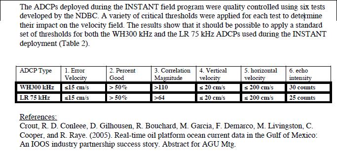
The teledyneSetQC.txt parameter file allows the user to change these parameters (speeds are in m/s). By default, chosen parameters are those which have been determined by Janet Sprintall for the RDI Workhorse Quartermaster ADCP 300kHz. See example below :
err_vel   = 0.15

pgood     = 50

cmag      = 110

vvel      = 0.2

hvel      = 2.0

ea_thresh = 30
However relevant thresholds need to be set for each dataset and no default set of thresholds can cover all possible datasets!
This test raises a warning if applied without CMAGn and ABSIn being vertically bin-mapped.
TimeSeries Spike Quality Control test - imosTimeSeriesSpikeQC - Optional
The IMOS TimeSeries Spike Quality Control Test provides both an automatic and interactive way to detect spikes in Time series.
The implementation of this test spans releases 2.6.6 (non-burst data) and 2.6.7 (burst data/interactivity) through the IMOSTimeSeriesSpikeQC function.
This general function allows one to detect spikes in both burst and non-burst data, with different tests and parameters, on a per variable basis. The selection of which spike test to use in each variable is handled by a UI element. Moreover, a preview option allows the operator to change test parameters and see results immediately.

The figure above shows a typical preview window of the imosTimeSeriesSpikeQC test for burst-data.
This method is optional. It's also particular in the sense that it can use other QC results, such as from InOutOfWaterQC, to clip the series and ignore invalid data that occurs continuously from the start and towards the end of the series. This clipping is done only with continuous invalid data, while any manual or intermittent bad QC values found in between are used within the QC test.
For Non-burst data, the following methods are available for spike classifications:
- Despiking1 - OTSU Thresholding with a Savitzky-Golay Filter.
This method works by applying the OTSU threshold method on the high-frequency portion of a signal. The high-frequency samples are computed by filtering out the low-frequency response with a Savitzky-Golay filter. Hence, the global OTSU threshold is computed only over a certain noise level, defined by the filter options. The Savitzky-Golay filter is a smoothing filter that uses a local least-squares polynomial approximation. It can be compared to a moving average, but with convolution weights defined by a polynomial. This dual-step method is used in the same way as the OTSU threshold.
The function requires four parameters:
a. An odd window - an odd integer to define the weight/coefficient distribution of the convolution. If even windows are provided, the nearest lower odd number is used.
b. Polynomial order - an integer to define the polynomial fit within the window (2-quadratic, 3-cubic, etc.)
c. Number of Histogram bins - an integer number of histogram bins for the OTSU threshold.
d. scale factor - a float to scale the OTSU threshold.
The naming convention was also kept. This method assumes that 1. the spike is contained within a (high) frequency band, 2. its amplitude is high and significant at the noise level, and 3. the spike is within the window. The method is useful to detect singleton spikes with high amplitude. However, the method may fail to detect small-amplitude spikes (given a global threshold), and is prone to false-positives, particularly if the signal is not smooth (sharp gradients relative to the window). The method is also not well-defined for non-equally spaced data. Bigger windows may also lead to no detections at the start/beginning of the time series.
The implementation of the filter was kept as originally provided, but with slight modifications and refactoring. These modifications are mostly to allow dynamical values for histogram bins and scale parameters (c,d). Original code was provided by Ken Ridgway. The figure below exemplifies the case where this classifier creates false-positives in the presence of noise. Some of the false-positives can still be removed by using a large window, but at the expense of a lower number of detections in other places.

- Despiking2 - OTSU Threshold method.
The method works by computing a threshold based on the inter variance of histogram bins. The threshold is global and based on the maximum inter-bin variance. The method is useful to split bi-modal data, and in its original form depends only on the number of histogram bins. The typical usage here is to binary split a population based on the threshold. Here, we mark all values above the computed threshold as a spike. The canonical reference for the method is Otsu1979, and usage is extensively reported in analytical chemistry and image processing literature.
The implementation here depends on three parameters:
a. Number of Histogram bins - an integer number of histogram bins.
b. Scale factor - a float weighting factor for the threshold.
c. Centralisation - a boolean switch to centralize/average consecutive values above the threshold
The naming convention (despiking2) was kept, with the addition of the algorithm name. The code was refactored from its original version and the centralisation was shifted from leftmost index to rightmost index, since the signal is differentiated (ceiling). The original code was provided by Ken Ridgway.
The method is useful for few and large amplitude spikes. In the presence of realistic signals, with trend and noise, the method usually fails for visible and limited amplitude spikes. The figure below shows how a simple global threshold, apart from detecting most spikes, still miss some relatively small amplitude ones.

- Hampel method.
This is a robust (in the statistical sense) method that uses the concept of a moving median over a window to compute the position and the median absolute deviation (MAD) for scale (variability). It's comparable to the dual-step method above, but using robust statistical moments with a local threshold (within a window). The robustness came from the ability of the estimators to be less sensitive to large variations within the window, and thus be less affected by outliers within the samples. Hence, the method is capable of identifying spikes of different amplitudes. For this reason, it's extensively used to filter spikes and instrument noise. A comparable method, although less robust, is the moving mean identifier. The canonical reference is Hampel1974, but a more practical reference is Liu2004
The implementation here is just a wrapper from the Matlab signal toolbox function hampel, although with extra parameters:
a. half window width - an integer defining the one-side window length.
b. mad factor - a scale for the mean absolute deviation which values above will be marked as a spike.
c. lower mad limit - a lower hard limit on the computed mad. MAD values below this are ignored.
The full window in the Hampel method is fullwindow = 1+2*half_window_width. The lower mad limit parameter may be useful to ignore very small deviations of the signal, such as when the signal variability is very low or close to the instrument precision range. However, the lower mad limit is an aposteriori limit and may cause some positive detections to be disregard. One may need to tune the lower mad limit to very low values together with the mad factor parameter.
The method is very useful to detect spikes with different amplitudes, even within the same window. Hence, it's widely used for outlier removal, given that it could easily substitute the offending outlier by a median of the respective window. Another advantage over the other methods is the wide range (sensitivity) of its parameters and their representativeness (clear intent). The method can also lead to false positives, particular if spikes are very close together in the window or if the mad factor is too low.
The figure below shows how the Hampel method may miss some spikes without proper parameter tuning. Increased detection rates may be possible without false-positives (the following figure).


For Burst data, the following methods are available for spike classifications:
- BurstHampel method.
This method is similar to the Hampel method in the non-burst data, although with extra parameters to customise the handling of burst data.
Parameters:
a. use burst window - a boolean to consider the window over burst numbers or over individual samples.
b. half window width - an integer defining the one-side window length (bursts or samples).
c. mad factor - a scale for the mean absolute deviation which values above will be marked as a spike.
d. lower mad limit - a lower hard limit on the computed mad. MAD values below this are ignored.
e. repeated only - a boolean to consider spikes only the repeated entries detected.
The implementation here allows three major operations over burst data - 1. individual burst handling, 2. consideration of ensemble of bursts, and 3. ignoring the burst spacing.
For individual burst handling, use_burst_window needs to be equals to 1 and half_window_width equals 0. This way, the Hampel method will be applied to every individual burst (sandboxed). This is useful to granularly mark spikes within bursts.
An ensemble of bursts is used if the same configuration above is changed to any positive integer over the half_window_width parameter, which will apply the window at burst level (e.g. half_window_width==1 will use all samples within the t-1,t,t+1 bursts). This is useful for example if an entire burst is a spike, or if one seeks to include more bursts on a window (all the samples in the bursts are considered). The last parameter repeated_only is useful here, and ignored otherwise, since when marshalling the window, one may seek to only include spikes that are found more than one time. This allows the filter to perform slightly better if sharp gradients in MAD are present.
Finally, to ignore the burst spacing, use_burst_window needs to be equal to 0. The half_window_width parameter is then considered to be the window in terms of samples (as in the Hampel method for non-burst data). This is useful if the number of burst samplings is high and the burst sampling interval is small (or could be ignored). The mad factor needs to be tuned to account for the burst-to-burst variability, however.
The method works faster if burst spacing is ignored since there is a considerable overhead of applying the same function sandboxed to a number of individual bursts. Unless one needs to be very granular and mark samples within a burst as spikes, tunning the scale parameter to account for the burst-to-burst variability and avoid using burst windows is very practical.
The figures below show the BurstHampel method detecting a singleton spike within a burst and an "entire burst as a spike" case.


- RunningStats method.
This method is a generalisation of the Running Statistical method implemented in the BurstQCStats branch. It's a simple function that marshals over every individual burst and computes a threshold with a scale (e.g. mean) and dispersion (e.g. standard_deviation) functions, marking everything above/below as a spike. The method differs slightly from the one in the BurstQCStats branch, however, since the burst detection here is more robust and this method can handle bursts with different lengths (if any). Finally, the implementation here permits the future development of further statistical operations at a granular/burst level, although currently available functions are limited (see below).
The overall parametrisation is:
threshold = scale_function(iburst) +- scale*dispersion_function(iburst)
The free parameters are:
a. scale function - a function handle to compute scale.
b. dispersion function - a function handle to compute dispersion.
c. dispersion factor - a scale for the dispersion.
The supported functions for scale are nanmean,nanmedian. Dispersion functions available are nanstd,mad_median,mad_mean. The naming mad_median/mad_mean is explicit to differentiate the median absolute deviation from the mean absolute deviation computations.
For compatibility with the BurstStatsQC branch, the operator needs to configure the scale function to be nanmean, the dispersion function to be nanstd, and the dispersion factor to be equal to 2. This was the typical filter applied to TEMP and PSAL. Note that a more robust behaviour can be reached by using the median/mad_median pair.
The figure below shows the same result as the BurstHampel method for an individual spike within a burst.

References:
Otsu, N., "A Threshold Selection Method from Gray-Level Histograms." IEEE Transactions on Systems, Man, and Cybernetics. Vol. 9, No. 1, 1979.
Hampel, F. R. "The Influence Curve and Its Role in Robust Estimation." Journal of the American Statistical Association 69, no. 346, 1974.
Liu, H. Shah, S., Jiang, W. , "On-line outlier detection and data cleaning", Computers & Chemical Engineering, Volume 28, Issue 9, 2004.