#!/usr/bin/env python
""" Examples of using qhull via scipy to generate 3D plots in visvis.
Requires numpy ver 1.5, scipy ver 0.9 and qhull from
http://www.qhull.org/ (on Windows this comes with Scipy).
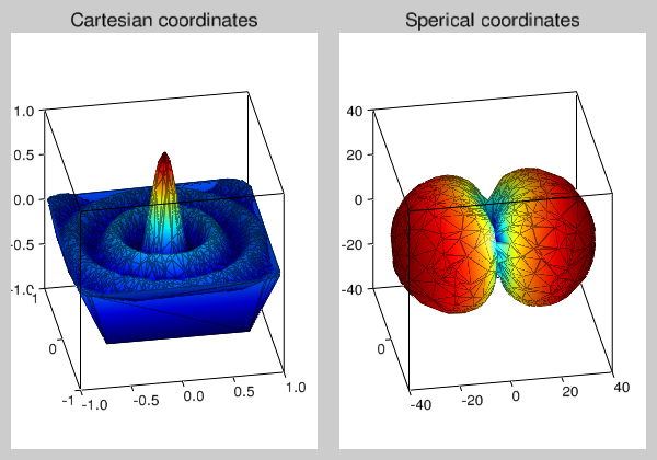
plot3D meshes and plots random convex transformable data in both cartesian
and spherical coordinates
Play around with the many input parameters to plot3D to make interesting plots.
Keith Smith, 4 March 2011
"""
import numpy as np
from scipy.spatial import Delaunay
import visvis as vv
def plot3D( vuvi,
coordSys='Cartesian',
raised = True,
depRange=[-40,0],
ambient = 0.9,
diffuse = 0.4,
colormap = vv.CM_JET,
faceShading='smooth',
edgeColor = (0.5,0.5,0.5,1),
edgeShading = 'smooth',
faceColor = (1,1,1,1),
shininess = 50,
specular = 0.35,
emission = 0.45 ):
""" plot3D(vxyz,
coordSys=['Cartesian', 'Spherical'],
raised = True,
depRange=[-40,0], #Note: second range limit not currently used
rangeR=[-40,0],
ambient = 0.9,
diffuse = 0.4,
colormap = vv.CM_JET,
faceShading='smooth',
edgeColor = (0.5,0.5,0.5,1),
edgeShading = 'smooth',
faceColor = (1,1,1,1),
shininess = 50,
specular = 0.35,
emission = 0.45 ))
"""
if coordSys == 'Spherical':
thetaPhiR = vuvi # data cols are theta, phi, radius
vxyz = np.zeros(vuvi.shape)
# Now find xyz data points on unit sphere (for meshing)
vxyz[:,0] = np.sin(thetaPhiR[:,0])*np.cos(thetaPhiR[:,1])
vxyz[:,1] = np.sin(thetaPhiR[:,0])*np.sin(thetaPhiR[:,1])
vxyz[:,2] = np.cos(thetaPhiR[:,0])
#normalize and scale dependent values
thetaPhiR[thetaPhiR[:,2] < depRange[0], 2] = depRange[0]
depVal = thetaPhiR[:,2] - np.min(thetaPhiR[:,2])
else:
vxyz = vuvi
vxyz[vxyz[:,2] < depRange[0], 2] = depRange[0]
numOfPts = np.shape(vxyz)[0]
depVal = vxyz[:,2]
# set to convex surface for meshing
# find center of data
center = np.average(vxyz, 0)
#center data
vxyz = vxyz - center
# find x-y plane distance to each point
radials = np.sqrt(vxyz[:,0]**2 + vxyz[:,1]**2)
# get max and adjust so that arctan ranges between +-45 deg
maxRadial = np.max(radials)/0.7
#get angle on sphere
xi = np.arctan2(radials / maxRadial, 1)
#force z axis data to sphere
vxyz[:,2] = maxRadial * np.cos(xi)
vxyz = np.append(vxyz, [[0.7, 0.7, -0.7],[-0.7, 0.7, -0.7],
[0.7, -0.7, -0.7],[-0.7, -0.7, -0.7]], axis=0)
# Send data to convex_hull program qhull
dly = Delaunay(vxyz)
meshIndx = dly.convex_hull
# Check each triangle facet and flip if
# vertex order puts back side out
for index, (I1, I2, I3) in enumerate(meshIndx):
a = vxyz[I1,:] - vxyz[I2,:]
b = vxyz[I2,:] - vxyz[I3,:]
c = np.cross(a, b)
if np.dot(c, vxyz[I2,:]) > 0:
meshIndx[index] = (I1, I3, I2)
# if 3D surface adjust dependent coordinates
if raised:
if coordSys == 'Spherical':
vxyz[:,0] = depVal*np.sin(thetaPhiR[:,0])*np.cos(thetaPhiR[:,1])
vxyz[:,1] = depVal*np.sin(thetaPhiR[:,0])*np.sin(thetaPhiR[:,1])
vxyz[:,2] = depVal*np.cos(thetaPhiR[:,0])
else:
vxyz = vxyz + center
vxyz[:numOfPts,2] = depVal
else:
if coordSys == 'Spherical':
depRange[0] = 1.0
else:
# Since qhull encloses the data with Delaunay triangles there will be
# a set of facets which cover the bottom of the data. For flat
# contours, the bottom facets need to be separated a fraction from
# the top facets else you don't see colormap colors
depValRange = np.max(vxyz[:numOfPts,2]) - np.min(vxyz[:numOfPts,2])
vxyz[:numOfPts,2] = vxyz[:numOfPts,2] / (10 * depValRange )
#normalize depVal for color mapping
dataRange = np.max(depVal) - np.min(depVal)
depVal = (depVal- np.min(depVal)) / dataRange
# Get axes
ax = vv.gca()
ms = vv.Mesh(ax, vxyz, faces=meshIndx, normals=vxyz)
ms.SetValues(np.reshape(depVal,np.size(depVal)))
ms.ambient = ambient
ms.diffuse = diffuse
ms.colormap = colormap
ms.faceShading = faceShading
ms.edgeColor = edgeColor
ms.edgeShading = edgeShading
ms.faceColor = faceColor
ms.shininess = shininess
ms.specular = specular
ms.emission = emission
ax.SetLimits(rangeX=[-depRange[0],depRange[0]],
rangeY=[-depRange[0],depRange[0]],
rangeZ=[-depRange[0], depRange[0]])
# Start of test code.
if __name__ == '__main__':
# Create figure
fig = vv.figure()
fig.position.w = 600
# Cartesian plot
numOfPts = 2000
scale = 1
# Create random points
xyz = 2 * scale * (np.random.rand(numOfPts,3) - 0.5)
# 2D sync function
xyz[:,2] = np.sinc(5*(np.sqrt(xyz[:,0]**2 + xyz[:,1]**2)))
#xyz[:,2] = scale - ( xyz[:,0]**2 + xyz[:,1]**2)
# Plot
vv.subplot(121)
vv.title('Cartesian coordinates')
plot3D(xyz, depRange=[-1,0])
#plot3D(xyz, depRange=[-1,0], raised=False)
# Sperical plot
numOfPts = 1000
# Create random points
ThetaPhiR = np.zeros((numOfPts,3))
ThetaPhiR[:,0] = np.pi * np.random.rand(numOfPts) # theta is 0 to 180 deg
ThetaPhiR[:,1] = 2 * np.pi * np.random.rand(numOfPts) # phi is 0 to 360 deg
ThetaPhiR[:,2] = 10 * np.log10((np.sin(ThetaPhiR[:,0])**4) * (np.cos(ThetaPhiR[:,1])**2))
# Plot
vv.subplot(122)
vv.title('Sperical coordinates')
plot3D(ThetaPhiR, coordSys='Spherical')
#plot3D(ThetaPhiR, coordSys='Spherical', raised=False)
# Run main loop
app = vv.use()
app.Run()