Satellite imaging - alabarga/geospatial-python GitHub Wiki
We will be working with earth-observing meteorological satellite instrument data. There are many different variations of how the data can be structured, what it physically represents, how it changes over time, and how it can be used in a particular type of application. The following is an overview of some common characteristics of meteorological satellite observations. We'll go in to a few details as we explore real data later on and completely ignore other details for simplicity.
Satpy operates on data from earth-observing satellite instruments. The data can be used to study changes in the atmosphere, vegetation, oceans, pollution, and many others.
Satellites can be in a high-altitude geostationary orbit or a lower altitude polar-orbiting orbit. Geostationary satellites typically provide observations at higher temporal rates of the same region faster (~30s in some), but usually have a lower spatial resolution and only see part of the Earth. Polar orbiters are usually at a higher spatial resolution and cover much more of the Earth, but it takes longer to get all of this coverage.
| Geostationary | Polar-orbiting |
|---|---|
Credit: Clayton Suplinski, SSEC, UW-Madison
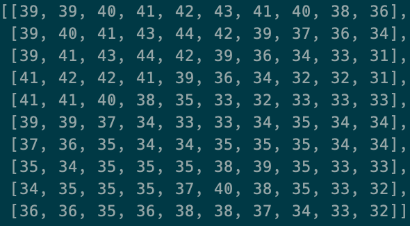
The instrument data we will be working with is imagery data; data from "imager" instruments. In most cases, these arrays of data points can be thought of as a 2D image of pixels.
|
→ |

|
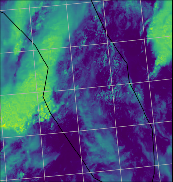
The data we will be looking at is geolocated. We need to be able to assign each pixel of data to a geographic region. Data footprints that can be somewhat difficult to describe are typically simplified by specifying only the center point and the pixel's radius or cell width. We may know the exact longitude and latitude coordinates of each pixel or we may be given a gridded version of the data where each pixel is spread uniformly across a rectangular area.
If you are familiar with projections, we'll get to those later.
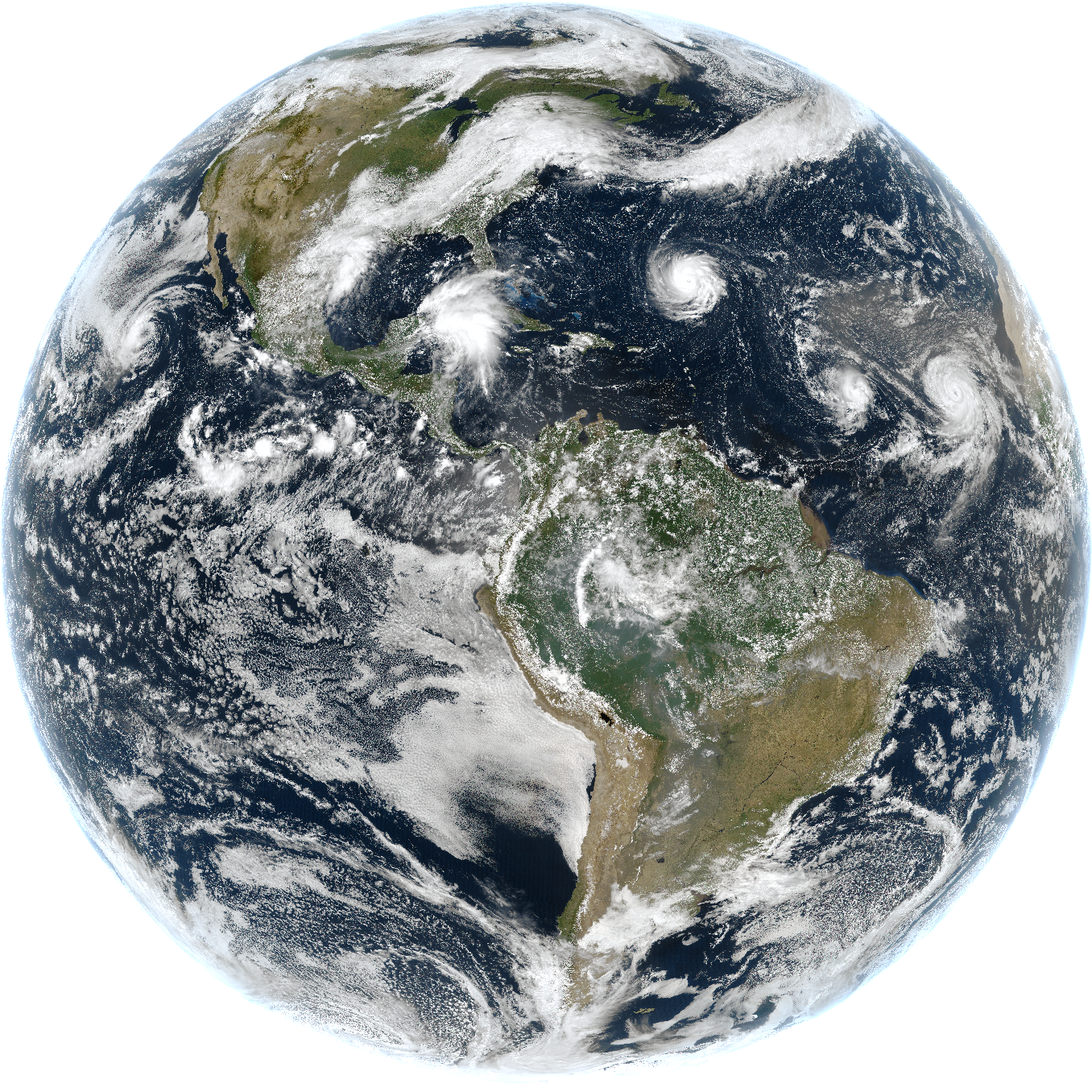
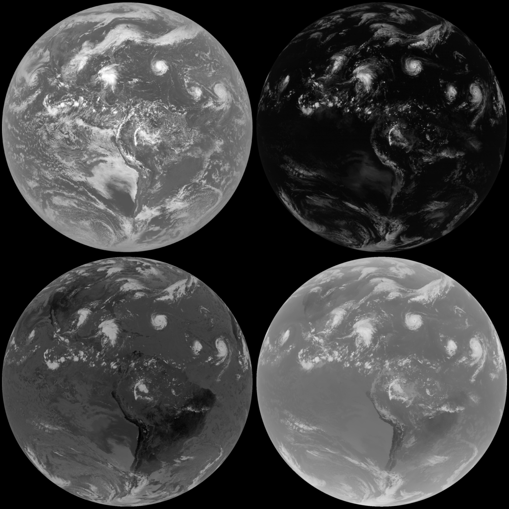
The satellite instrument data we will be working with are a collection of radiation measurements. By taking individual measurements of the radiation reflected or emitted by objects on Earth, we can get a good snapshot of the Earth from space. Satellite instruments will typically have multiple bands or channels where each one measures a specific wavelength of the electromagnetic spectrum. Each band can show us something different about the Earth.
Some geostationary satellites record data for different sectors or regions of the Earth depending on their purpose and design. For example the GOES-16 ABI instrument has 4 sectors:
- Full Disk (FD or FLDK)
- Continental United States (CONUS)
- Mesoscale 1 (M1)
- Mesoscale 2 (M2)
The below image shows these different sectors and how quickly GOES-16 ABI records data for them. The colors on the image indicate how much of the Earth each data pixel measures.
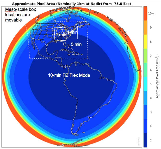
Credit: Mat Gunshor, CIMSS
Satellite imagery is a measurement of reflectance from the earth’s surface (or how effective the earth is at reflecting light and other radiant energy). Behind each raw pixel, there is a number that relates to the bands on the electromagnetic spectrum. The electromagnetic spectrum. Credit: NASA
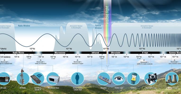
While the bands measured can cover a very large range of light reflecting that is imperceptible to the human eye, the most commonly thought of satellite imagery is natural colour imagery, or imagery that measures the visible spectrum. However, combining bands in different ways beyond natural colour can reveal many different things about the surface.