ComparisonOtherCodes - adda-team/adda GitHub Wiki
Many researchers have used ADDA and compared it with other codes based on DDA or other light scattering methods. The purpose of this page is to give a few representative examples instead of providing a full overview. Figures on this page are either in vector format (svg) or can be clicked to open a larger image.
- Other DDA codes
- Multiple multipole program (Gaussian beam)
- Null-field method with discrete sources (anisotropic material)
- Finite difference time domain method
- Pseudo-spectral time domain method
- Improved geometric optics method
- Tsym for cubes
- Particles near surface
- Decay rate enhancements
- Inhomogeneous anisotropic sphere
- Aggregate of spheres
- References
Comparison of four different DDA codes, including ADDA 0.7a and DDSCAT 6.1, was performed by (Penttilä et al. 2007) for simulation of different wavelength-sized particles both in single orientation and averaged over all orientations. Here we present a brief summary and a few sample results from this paper. ADDA is faster than other codes by a factor of 2.3 to 16 and it is the least memory consuming code. Results of simulations of light scattering by a sphere in a fixed orientation are shown in the following figure. All scatterers considered in this section have volume-equivalent size parameter 5.1 and refractive index 1.313. SIRRI and ZDD denote codes by Simulintu Oy in Finland and Zubko and Shkuratov respectively. All codes result in almost identical relative error of S11(θ), as compared with the Mie theory, showing that the codes use the same formulation of DDA, except SIRRI that is slightly different.

On contrary, orientation averaging schemes of the codes are different. Orientation averaged results for a randomly constructed aggregate of 50 spheres are shown in the next figure (here and below reference results are obtained using the T-matrix method). One can see that results differ, and the errors of ADDA results are the largest. That is explained by the fact that for ADDA we used 16×9×8 sample points for Euler angles α, β, and γ respectively. Other codes used less α sample angles (11, 4, and 1) but more β and γ sample angles, resulting in approximately the same total number of sample angles. Therefore, ADDA is faster at expense of possible deterioration of accuracy. However, for other asymmetric particles studied in (Penttila et al. 2007) ADDA results in comparable to other codes accuracy even with current settings (particle showed here was the least favorable for ADDA).

The results for axisymmetric particles are principally different. Here we consider only a prolate spheroid with aspect ratio 2 (see the next figure). One can see that ADDA result (the first curve) is much less accurate than other codes. The accuracy of ADDA is unusually bad, even compared to the previous figure. In the following we explain this fact. For axisymmetric particles the dipole array is symmetric with respect to 90° rotation over the symmetry axis. Moreover, the range from 0° to 90° for γ is mirror symmetric with respect to the 45°. Hence, the most efficient way of orientation averaging for such particles is to sample γ uniformly in the range from 0° to 45°, and also to use less γ sample angles but more β sample angles. Sampling by other codes satisfies these conditions. The situation for ADDA is remarkably different. 8 γ angles are used, which are spaced with interval 45°, hence they map in only two distinct angles (0° and 45°) inside the reduced range. That means that for axisymmetric particles ADDA repeats calculation for four equivalent sets of orientations. Moreover, Romberg integration, which is a higher order method, performs unsatisfactory when applied to a range that contains several periods of the periodic function to be integrated and only a few points per each period. An analogous discussion applies to the β angle since both spheroid and cylinder have a symmetry plane perpendicular to the symmetry axis.

It is important to note that ADDA is perfectly suitable to calculate orientation averaging of axisymmetric particles efficiently, but it requires a user to manually modify the sampling intervals for Euler angles in the input files. For instance, for the discussed scatterers the choice of 17 β angles from 0° to 90° and 5 γ angles from 0° to 45° is appropriate. The result of this tuned orientation averaging for spheroid, obtained using ADDA 0.76, is shown as the last curve in the previous figure. It requires about 20% more computational time than the initial scheme, but still it is significantly faster than other codes. One can see that its accuracy is comparable to or even better than that of other codes. This result was not included in (Penttila et al. 2007), because such modifications of the input files were considered a ‘fine-tuning’. DDSCAT may also benefit from reduction of angle ranges, but in much lesser extent (in these particular cases).
Therefore, we may conclude that ADDA is clearly superior for particles in single orientation. Its orientation averaging scheme is not that flexible, especially when small number of sample angles is used. However, in most cases it results in accuracy not worse than that of other codes, if particle symmetries are properly accounted for. Moreover, inflexibility is compensated by the adaptability of the ADDA orientation averaging scheme and its ability to estimate the averaging error. We should also note, that the optimal strategy for orientation averaging is still an open question (see e.g. #40).
Finally, the described comparison is already outdated. Both ADDA and DDSCAT have undergone significant improvement since that time. Moreover, a new code OpenDDA have been released, claiming superior computational efficiency.
To validate the part of ADDA, which simulates scattering by a Gaussian beam, we conducted a simple test and compared results with that of the multiple multipole program. The latter were provided by Roman Schuh and Thomas Wriedt. Sphere with size parameter 5 and refractive index 1.5 is illuminated with a Gaussian beam with wavelength 1 µm, width 2 µm, and position of the beam center (1,1,1) µm. The beam propagates along the z-axis. We calculated S11(θ) in the yz-plane, scattering angle θ was considered from the z-axis to the y-axis. We used 64 voxels per diameter of the sphere. ADDA 0.76 was used with a command line:
adda -grid 64 -lambda 1 -size 1.59155 -beam barton5 2 1 1 1 -ntheta 180
The results are shown in the following figure, indicating perfect agreement between two methods.

(Schmidt and Wriedt 2009) extended the null-field method with discrete sources (NFM-DS) to anisotropic scatterers and verified their code by comparison with ADDA and DDSCAT. The following figure shows one particular example for ellipsoid with semi-axes ka=2, kb=3, kc=4 (k is the wavenumber) and refractive index mx=1.5, my=mz=1.1. Incident wave propagates along the z-axis and S11 is calculated in xz-plane. NFM-DS data was provided by Vladimir Schmidt. ADDA 0.79 was run with the following command line.
adda -size 4 -shape ellipsoid 1.5 2 -m 1.5 0 1.1 0 1.1 0 -anisotr -orient 90 0 0
where the last option (-orient) was used for convenience to make the first two columns of the file mueller produced by ADDA (corresponding to yz-plane in particle reference frame) equivalent to the sought S11 in xz-plane in laboratory reference frame.

A systematic comparison of DDA and the finite difference time domain (FDTD) method was performed for large dielectric scatterers by (Yurkin et al. 2007). Here we summarize these results. Simulations were performed for spheres with size parameter x from 20 to 80 and refractive index m from 1.02 to 2 (all m also had a fixed negligible imaginary part). Since both methods are potentially exact if infinite discretization is employed, a certain accuracy was required – relative error of Qext less than 1% and the root-mean-square relative error of S11 over the whole range of θ less than 25%. Then simulation times were compared. ADDA v.0.76 was used as DDA implementation, and FDTD implementation was developed in the Biomedical Laser Laboratory at East Carolina University, based on the algorithms described by Yang and Liou with numerical dispersion correction.
The main conclusion is summarized in the following figure, where a ratio of computational times of two methods is shown versus x for different m. DDA is more than an order of magnitude faster for m ≤1.2 and x>30, while for m ≥1.7 FDTD is faster by the same extent. m=1.4 is a boundary value, for which both methods perform comparably. The DDA errors of S11(θ) for m=1.02 are mostly due to the shape errors, which are expected to be smaller for rough and/or inhomogeneous particles. Simulations for a few sample biological cells lead to the same conclusions. Although these conclusions depend on particular scattering quantity and on the implementations of both methods, they will not change principally unless a major improvement of one of the method is made. However, for general complex refractive indices the results of the comparison are expected to be significantly different.

A systematic comparison of DDA and the pseudo-spectral time domain (PSTD) method was performed for large dielectric scatterers by (Liu et al. 2012). Here we summarize these results. Overall method of comparison was analogous to that for FDTD. Simulations were performed for spheres with size parameter x from 10 to 100 and refractive index m from 1.2 to 2. The following accuracy was required – relative error of Qext less than 1% and the root-mean-square relative error of S11 over the whole range of θ less than 25%. Then simulation times were compared. ADDA v.0.79 with the default settings was used as the DDA implementation, and the PSTD implementation was developed in the Department of Atmospheric Sciences of Texas A&M University.
The main conclusion is summarized in the following figure, where the regions of superiority of DDA and PSTD are shown. Differences of the simulation times (to reach the same accuracy) were up to a factor of 100 (both ways). Simulations for a few sample spheroidal particles lead to the same conclusions.

Although these conclusions depend on particular scattering quantity and on the implementations of both methods, they will not change principally unless a major improvement of one of the method is made. In particular, we have tried to push ADDA to the limit for two spheres (x=10, m=2 and x=80, m=1.2). We tried different DDA formulations and iterative solvers, resulting in 14 and 4 times decrease of computational time for these two cases, respectively. However, these times were still two-three times larger than that of PSTD. However, for general complex refractive indices and/or inhomogeneous particles the results of the comparison are expected to be significantly different.
In particular, more recently (Podowitz et al. 2014) considered refractive index of ice in a wide spectral range (including absorbing ones). It was shown that absorption improves the performance of both methods, however, DDA especially benefits from it. For strongly absorbing ice (Im(m)>0.1) DDA is about twice faster than PSTD for all tested size parameters (up to 100).
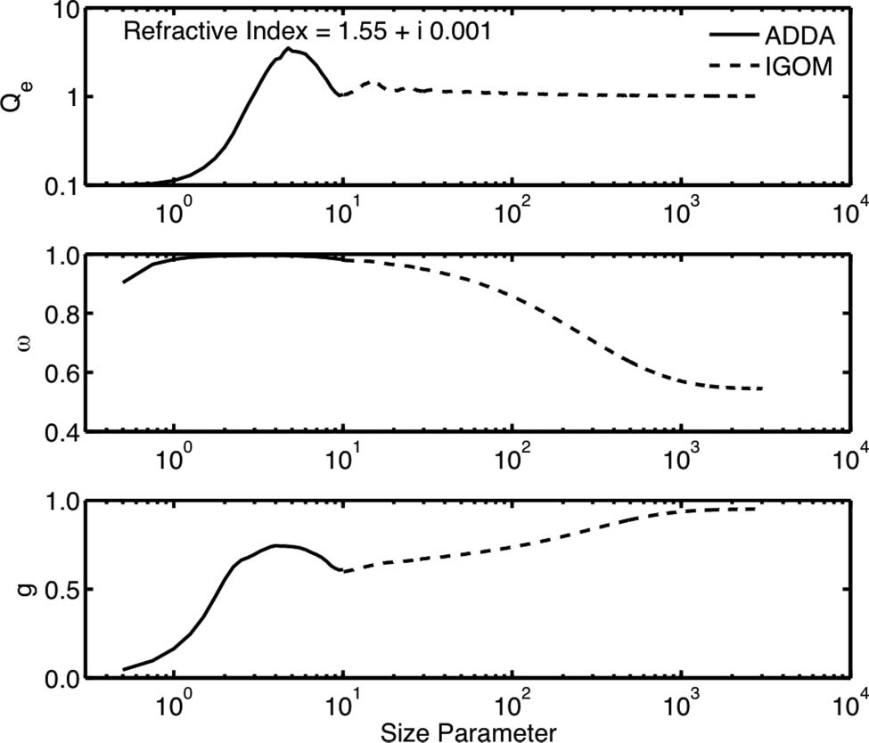
ADDA was compared with the improved geometric optics method (IGOM) for simulation of randomly-oriented ellipsoids (Bi et al. 2009) and hexahedra (Bi et al. 2010). The accuracy of ADDA was assumed good enough (unfortunately, the details of the DDA simulations were not specified), while accuracy of IGOM is tested against it. A particular example from (Bi et al. 2010) is shown in the following figure, depicting integrated scattering properties of randomly oriented nonsymmetric hexahedra versus the size parameter. One can see that both methods agree in intermediate size parameter range, thus effectively closing the gap between geometric-optics and wave-optics methods. However, the deviations for angle-resolved light scattering properties ,e.g. S11, can still be significant.
ADDA was compared with Tsym, a T-matrix code employing discrete symmetries of the scatterer, for a number of cubes with kD=0.1 and 8 (k is the wavenumber, D is the cube edge) and refractive index m=1.6+0.01i, 0.1+i, and 10+10i (Yurkin and Kahnert 2013), pushing the accuracy of both codes to the limit. Here we present only the results for one case – kD=8 and m=1.6+0.01i. The cube is in fixed orientation with edges along the axes. ADDA v.0.78.2 was used with default settings, except for the FCD formulation and 10−10 convergence threshold for the iterative solver. The command line was the following:
adda_mpi -size 8 -m 1.6 0.01 -ntheta 180 -shape box -int fcd -pol fcd -eps 10 -grid <nx>
where 5 grid sizes (<nx>) were used from 256 to 512, and extrapolation technique (Yurkin et al. 2006) was employed afterwards. Also, a special technique was used for Tsym results to estimate computational accuracy. Results for the integral scattering quantities are summarized in the following table. Uncertainties (±) are in the last shown digits of the corresponding value and have nominal confidence level of 95%.
| Qext | Qsca | Qabs | |
|---|---|---|---|
| ADDA | 4.2480442 ± 3 | 3.9715646 ± 3 | 0.2764796 ± 1 |
| Tsym | 4.24775 ± 33 | 3.97156 ± 24 | 0.2757 ± 7 |
Below is the results for intensity I=S11 in the yz-plane, showing relative differences between the two methods and their internal error estimates.

To validate the part of ADDA, which implements simulation of optical properties of particles near surface, we compared it with a number of other methods.
First test is for Fe prolate spheroid (semi-axes 25nm and 50nm, refractive index 1.35+1.97i) placed on Si substrate (refractive index 4.37+0.08i), illuminated by plane wave from above propagating at 45° relative to the surface normal. Wavelength is 488nm. ADDA v.1.3b2 (r1266) was used with a command line
adda -shape ellipsoid 1 2 -size 0.05 -lambda 0.488 -surf 0.05 4.37 0.08 -m 1.35 1.97 -grid <nx> -prop 1 0 -1 -ntheta 180
where <nx> varied between 16 and 64. Shown below is normalized (to have maximum value of 1) perpendicular and parallel (to scattering plane) scattering intensities. Scattering angle corresponds to the spherical angle θ of laboratory reference frame inside the main scattering plane (given by incident and reflected direction).

Reference results are T-matrix simulations, digitized from Fig.4.7 of (Doicu et al. 2008) with appropriate modification of scattering angle definition. The agreement is perfect for perpendicular intensity, but there are some discrepancies for parallel. The latter, however, clearly diminish with refining discretization, and the remaining difference is comparable to that between the T-matrix and discrete-sources-method in (Doicu et al. 2008) (data not shown).
A second test is for Ag sphere (radius R=50nm, refractive index 0.25+3.14i) placed on glass substrate (refractive index ms=1.5), illuminated by plane wave from below propagating at 60° relative to the surface normal (evanescent illumination). Wavelength is 488nm. ADDA v.1.3b4 was used with command line
adda -size 0.1 -lambda 0.488 -surf 0.05 1.5 0 -m 0.25 3.14 -prop 1 0 0.577350 -ntheta 180 -grid 64
Shown below are perpendicular and parallel scattering intensities (S11−S12 and S11+S12 respectively) in the main scattering plane.

Reference T-matrix results were provided by Vladimir Schmidt (calculated using NFM-DS) and coincide with that in Fig.4.10 of (Doicu et al. 2008). The former raw results were multiplied by a factor π(kR)2/ms, where k is the free-space wavenumber.
The test data for this section were provided by Stefania D'Agostino. The goal is to validate the part of ADDA, related to the point-dipole incident field, by comparing it with exact electromagnetic theory (EET) for a silver sphere (diameter 10 nm). EET is described in (Mertens et al. 2007), and the data were calculated with the online applet. The refractive index of silver is from Palik (Lynch and Hunter 1985) with linear interpolation. First, the decay-rate enhancements (total as well as radiative and non-radiative parts) at the wavelength of 354nm were calculated as a function of dipole distance from sphere surface for parallel and perpendicular orientations of the dipole with respect to sphere surface. ADDA v.1.3b4 was used with a command line
adda -beam dipole 0 0 <z> -prop <ori> -size 10 -lambda 354 -m 0.20959 1.43592 -sym enf -grid 160
where <z> is the distance from dipole to sphere center (in nm), i.e. distance from surface + 5, and <ori> is "1 0 0" or "0 0 1" for parallel and perpendicular orientations of the dipole respectively. The results are similar to Fig.1 of (D’Agostino et al. 2013), which were obtained with a previous version of ADDA using a number of code hacks and workarounds. Now only ADDA itself is required for such simulations.

Second, convergence of the results with refining discretization was studied for total decay-rate enhancement for a dipole (in two orientations) at 5 nm from the sphere surface as a function of the wavelength. The command line is
adda -beam dipole 0 0 10 -prop <ori> -size 10 -lambda <lam> -m <mre> <mim> -sym enf -grid <nx>
where <nx> is either 80 or 160, <lam> is the wavelength (in nm), and <mre> and <mim> are the corresponding real and imaginary parts of the refractive index.

The agreement with EET becomes better with refining discretization. Moreover, if we use the simplest Richardson-type extrapolation of the DDA results to zero voxel size, see (Yurkin et al. 2006) for justification, i.e. 2×(result for nx=160) − (result for nx=80), the agreement (green vs. blue line in the figure) is almost perfect (mostly within the line width).
A new method was developed to simulate light scattering by spheres with radially varying anisotropic dielectric permittivity (Zouros and Kokkorakis 2015). It solves the electric-field volume-integral equation using Dini-type spherical basis functions. It was compared with ADDA for a sphere with size parameter ka=π and the following diagonal permittivity tensor: εxx(r) = εyy(r) = 4/[1+(r/a)2], εzz(r) = [4−(r/a)2].
For DDA simulations the sphere was divided into nL 1-voxel-wide layers, each having a constant permittivity equal to its value at the layer middle. ADDA 1.3b4 was modified (recompiled) to support up to 192 different values of refractive index (up to 64 anisotropic layers). The command line is like
adda -lambda 1 -size 1 -shape read 64layers.geom -ntheta 180 -sym enf -anisotr -m <mxx1> 0 <myy1> 0 <mzz1> 0 ... <mzz64> 0
where both shape file and the list of different refractive indices was generated by a separate program. The following comparison results are adapted from Fig.7 of (Zouros and Kokkorakis 2015).

The agreement improves with increasing the number of layers. Moreover, if we use the simplest Richardson-type extrapolation of the DDA results to zero layer (voxel) size, see (Yurkin et al. 2006) for justification, i.e. 2×(result for nL=64) − (result for nL=32), the agreement (green vs. blue line in the figure) is almost perfect (mostly within the line width).
In the framework of the workshop "One-Billion-Particle Problem" several numerically exact codes (ADDA, multiple-sphere T-matrix – MSTM, fast superposition T-matrix method – FaSTMM, discrete exterior calculus – DEC) were compared with several radiative-transfer(RT)-type approximations (RT-CB, RT-CB-ic, R2T2) – see (Penttilä et al. 2021) for details. The test particles were aggregates consisisting of a lot of spheres with size parameter 1.76 and refractive index 1.5 + 0.0001i, packed with volume fraction 20%. In the following the results for 100 000 spheres (aggregate size parameter equal to 140) are discussed.
For DDA simulations a single random aggregate was used, the corresponding shape file was prepared beforehand. Ensemble averaging was replaced by orientation averaging, for which 512 steps over Euler angle α were used (cheap to compute), but only 9 steps over the angles β and γ (in total 58 orientations requiring separate simulations). ADDA 1.3b4 was executed with a command line:
adda_mpi -m 1.5 0.0001 -shape read 1h_10dpl.geom -dpl 10.0 -ntheta 1800 -eps 2 -orient avg avg-all.dat
The correspoding computational complexity is discussed in LargestSimulations. The results for intensity and degree of linear polarization (DOLP) versus scattering angles are shown below (part of Fig.2 from Penttilä et al. 2021). The forward-scattering region is excluded, since it is not adequately described by RT methods.

There is almost perfect agreement between numerically exact codes for the intensity, while the differences in DOLP are within the uncertainties of each method (that can be judged by the corresponding oscillations).
- Bi L., Yang P., Kattawar G.W., and Kahn R. Modeling optical properties of mineral aerosol particles by using nonsymmetric hexahedra, Appl. Opt. 49, 334–342 (2010).
- Bi L., Yang P., Kattawar G.W., and Kahn R. Single-scattering properties of triaxial ellipsoidal particles for a size parameter range from the Rayleigh to geometric-optics regimes, Appl. Opt. 48, 114–126 (2009).
- D’Agostino S., Della Sala F., and Andreani L.C. Dipole-excited surface plasmons in metallic nanoparticles: Engineering decay dynamics within the discrete-dipole approximation, Phys. Rev. B 87, 205413 (2013).
- Doicu A., Schuh R., and Wriedt T. Scattering by particles on or near a plane surface, Light Scattering Reviews 3, ed. Kokhanovsky A.A., Springer, Berlin, pp. 109–130 (2008).
- Liu C., Bi L., Panetta R.L., Yang P., and Yurkin M.A. Comparison between the pseudo-spectral time domain method and the discrete dipole approximation for light scattering simulations, Opt. Express 20, 16763–16776 (2012).
- Lynch D.W. and Hunter W.R. Comments on the optical constants of metals and an introduction to the data for several metals, Handbook of Optical Constants of Solids, ed. Palik E.D., Academic Press, San Diego, pp. 275–267 (1985).
- Mertens H., Koenderink A., and Polman A. Plasmon-enhanced luminescence near noble-metal nanospheres: Comparison of exact theory and an improved Gersten and Nitzan model, Phys. Rev. B 76, 115123 (2007).
- Penttila A., Zubko E., Lumme K., Muinonen K., Yurkin M.A., Draine B.T., Rahola J., Hoekstra A.G., and Shkuratov Y. Comparison between discrete dipole implementations and exact techniques, J. Quant. Spectrosc. Radiat. Transfer 106, 417–436 (2007).
- Podowitz D.I., Liu C., Yang P., and Yurkin M.A. Comparison of the pseudo-spectral time domain method and the discrete dipole approximation for light scattering by ice spheres, J. Quant. Spectrosc. Radiat. Transfer 146, 402–409 (2014).
- Schmidt V. and Wriedt T. T-matrix method for biaxial anisotropic particles, J. Quant. Spectrosc. Radiat. Transfer 110, 1392–1397 (2009).
- Yurkin M.A., Hoekstra A.G., Brock R.S., and Lu J.Q. Systematic comparison of the discrete dipole approximation and the finite difference time domain method for large dielectric scatterers, Opt. Express 15, 17902–17911 (2007).
- Yurkin M.A. and Kahnert M. Light scattering by a cube: accuracy limits of the discrete dipole approximation and the T-matrix method, J. Quant. Spectrosc. Radiat. Transfer 123, 176–183 (2013).
- Yurkin M.A., Maltsev V.P., and Hoekstra A.G. Convergence of the discrete dipole approximation. II. An extrapolation technique to increase the accuracy, J. Opt. Soc. Am. A 23, 2592–2601 (2006).
- Zouros G.P. and Kokkorakis G.C. Electromagnetic scattering by an inhomogeneous gyroelectric sphere using volume integral equation and orthogonal Dini-type basis functions, IEEE Trans. Antennas Propag. 63, 2665–2676 (2015).
- Penttilä A., Markkanen J., Väisänen T., Räbinä J., Yurkin M.A., and Muinonen K. How much is enough? The convergence of finite sample scattering properties to those of infinite media, J. Quant. Spectrosc. Radiat. Transfer 262, 107524 (2021).