Matrices and vectors

Declaring and using matrices in the Accord.NET Framework does not require much. In fact, it does not require anything else that is not already present at the .NET Framework. If you already have working code that uses another library, you don't have to convert your matrices to a different format. This is because Accord.NET is built to interoperate with other libraries and existing solutions, relying solely on default .NET structures to work.

To begin, please add the following using directive on top of your .cs (or equivalent) source code file:

using Accord.Math;

After this, all .NET numeric types will be extended with mathematical methods.

Matrix operations in the Accord.NET Framework through extension methods.

Declaring and creating matrices and vectors

The most straightforward way to declare a matrix in Accord.NET is simply using:

 double[,] matrix = 
 {
    { 1, 2 },
    { 3, 4 },
    { 5, 6 },
};

Yep, that's right. You don't need to create any fancy custom Matrix classes or vectors to make Accord.NET work, which is a plus if your code uses other libraries. You are also free to use both the multidimensional matrix syntax above or the jagged matrix syntax below:

 double[][] matrix = 
 {
    new double[] { 1, 2 },
    new double[] { 3, 4 },
    new double[] { 5, 6 },
};

Special purpose vectors can also be created through specialized methods. Those include vector indices

int[] indices1 = Vector.Range(5);      // { 0, 1, 2, 3, 4 }
int[] indices2 = Vector.Range(2, 10);  // { 2, 3, 4, 5, 6, 7, 8, 9 }

and interval vectors

double[] interval = Vector.Interval(-2.0, 4.0); // { -2, -1, 0, 1, 2, 3, 4 };

and some notable matrices like

double[,] I = Matrix.Identity(3);     // creates a 3x3 identity matrix
double[,] magic = Matrix.Magic(5);    // creates a magic square matrix of size 5

double[] ones = Matrix.Vector(5, 1.0);   // generates { 1, 1, 1, 1, 1 }
double[,] diagonal = Matrix.Diagonal(v); // matrix with v on its diagonal

double[,] A = Matrix.Identity(3).Multiply(2);
double[,] B = Matrix.Diagonal(3, 2.0);

Vector operations and properties

Albeit being simple double[] matrices, the framework leverages .NET extension methods to support all basic matrix operations.

double[] v = { 4, 5, 6 };

double[] a = v.Multiply(2);     // v .* 2: { 8,  10,  12 }
double[] b = v.Divide(2);       // v ./ 2: { 2,  2.5,  3 }
double[] c = v.Pow(2);          // v .^ 2: { 16,  25, 36 }

Operations include common products such as the dot, the outer, the Kronecker and the Cartesian products.

  // Declare two vectors
  double[] u = { 1, 6, 3 };
  double[] v = { 9, 4, 2 };

  // Products between vectors
  double inner = u.Dot(v);                // 39.0
  double[,] outer = u.Outer(v);           // 
  double[] kronecker = u.Kronecker(v);    // { 9, 4, 2, 54, 24, 12, 27, 12, 6 }
  double[][] cartesian = u.Cartesian(v);  // all possible pair-wise combinations

  // Addition
  double[] addv = u.Add(v);               // { 10, 10, 5 }
  double[] add5 = u.Add(5);               // {  6, 11, 8 }

  // Elementwise operations
  double[] abs = u.Abs();                 // { 1, 6, 3 }
  double[] log = u.Log();                 // { 0, 1.79, 1.09 }

  // Apply *any* function to all elements in a vector
  double[] cos = u.Apply(Math.Cos);       // { 0.54, 0.96, -0.989 }
  u.Apply(Math.Cos, u);                   // can also do optionally in-place

You can also perform operations between vectors and matrices:

  double[] v = { 9, 4, 2 };

  // Declare a matrix
  double[,] m =
  {
      { 0, 5, 2 },
      { 2, 1, 5 }
  };

  // Extract a subvector from v:
  double[] vcut = v.Get(startRow: 0, endRow: 2);  // { 9, 4 }

  // Some operations between vectors and matrices
  double[] Mv = m.Dot(v);                         // { 24, 32 }
  double[] vM = vcut.Dot(m);                      // { 8, 49, 38 }

  // Some operations between matrices
  double[,] Md = m.DotWithDiagonal(v);            // { { 0, 20, 4 }, { 18, 4, 10 } }
  double[,] MMt = m.DotWithTransposed(m);         // { { 29, 15 },   { 15, 30 }    }

Please note this is by no means an extensive list; please take a look on all members available on this class or (preferably) use IntelliSense to navigate through all possible options when trying to perform an operation.

Matrix operations and properties

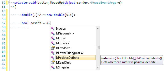
You can use the framework to compute some matrix properties:

// 3.1 Calculating the determinant
double det = A.Determinant();

// 3.2 Calculating the trace
double tr = A.Trace();

// 3.3 Computing the sum vector
{
    double[] u = { 1, 6, 3 };

    // 3.3.1 Computing the total sum of elements
    double sum = u.Sum();

    // 3.3.2 Computing the sum along the rows
    double[] sumVector = A.Sum(0); // Equivalent to Octave's sum(A, 1)

    // 3.3.2 Computing the sum along the columns
    sumVector = A.Sum(1); // Equivalent to Octave's sum(A, 2)
}

and also perform a number of matrix operations:

{
    // 2.1 Addition
    var C = A.Add(B);

    // 2.2 Subtraction
    var D = A.Subtract(B);

    // 2.3 Multiplication
    {
        // 2.3.1 By a scalar
        var halfM = A.Multiply(0.5);

        // 2.3.2 By a vector
        double[] m = A.Dot(new double[] { 1, 2, 3 });

        // 2.3.3 By a matrix
        double[,] M = A.Dot(B);

        // 2.4 Transposing
        double[,] At = A.Transpose();
    }
}


// 2.5 Elementwise operations

// 2.5.1 Elementwise multiplication
double[,] E = Elementwise.Multiply(A, B); // A.*B

// 2.5.1 Elementwise division
double[,] D = Elementwise.Divide(A, B); // A./B

Linear Algebra

You can use the framework to solve linear algebra problems:

// 4.1 Computing the inverse
var invA = A.Inverse();

// 4.2 Computing the pseudo-inverse
var pinvA = A.PseudoInverse();

// 4.3 Solving a linear system (Ax = B)
var x = A.Solve(B);

Matrix decompositions

One common task in matrix manipulation is to decompose a matrix into various forms. Some examples of the decompositions supported by the framework are listed below. Those decompositions can be used to solve linear systems, compute matrix inverses and pseudo-inverses and extract other useful information about data.

Decompositions	Multidimensional	Jagged
Cholesky	(double)(float)(decimal)	(double)(float)(decimal)
Eigenvalue (EVD)	(double)(float)
Generalized Eigenvalue [1]	(double)
Nonnegative Factorization	(double)
LU	(double)(float)(decimal)	(double)(float)(decimal)
QR	(double)(float)(decimal)
Singular value (SVD)	(double)(float)

Below are some examples on how to use the decompositions.

// Singular value decomposition
{
    SingularValueDecomposition svd = new SingularValueDecomposition(A);
    var U = svd.LeftSingularVectors;
    var S = svd.Diagonal;
    var V = svd.RightSingularVectors;
}
// or (please see documentation for details)
{
    SingularValueDecomposition svd = new SingularValueDecomposition(A.Transpose());
    var U = svd.RightSingularVectors;
    var S = svd.Diagonal;
    var V = svd.LeftSingularVectors;
}

// Eigenvalue decomposition
{
    EigenvalueDecomposition eig = new EigenvalueDecomposition(A);
    var V = eig.Eigenvectors;
    var D = eig.DiagonalMatrix;
}

// QR decomposition
{
    QrDecomposition qr = new QrDecomposition(A);
    var Q = qr.OrthogonalFactor;
    var R = qr.UpperTriangularFactor;
}

// Cholesky decomposition
{
    CholeskyDecomposition chol = new CholeskyDecomposition(A);
    var R = chol.LeftTriangularFactor;
}

// LU decomposition
{
    LuDecomposition lu = new LuDecomposition(A);
    var L = lu.LowerTriangularFactor;
    var U = lu.UpperTriangularFactor;
}

Loading and parsing from text

The framework can load any MATLAB-compatible .mat file using the MatReader class. It can also parse matrices written in MATLAB, Octave, Mathematica and C#/NET formats directly from text. Examples are shown below.

// From free-text format
double[,] a = Matrix.Parse(@"1 2
                             3 4");

// From MATLAB/Octave format
matrix[,] b = Matrix.Parse("[1 2; 3 4]", OctaveMatrixFormatProvider.InvariantCulture);

// From C# multi-dimensional array format
string str = @"double[,] matrix = 
               {
                  { 1, 2 },
                  { 3, 4 },
                  { 5, 6 },
               }";

double[,] c = Matrix.Parse(str, CSharpMatrixFormatProvider.InvariantCulture);

Numeric optimization

Another very common task in mathematics, machine learning and statistics is the need to optimize (i.e. find the maximum or minimum) of a function. The Accord.Math.Optimization namespace contains classes for constrained and unconstrained optimization, such as for example Levenberg-Marquardt, (Conjugate Gradient) (CG), Broyden–Fletcher–Goldfarb–Shanno (BFGS) and the Bounded Broyden–Fletcher–Goldfarb–Shanno (Bounded-BFGS) for unconstrained optimization; the Goldfarb-Idnani solver for Quadratic Programming (QP) problems, the Augmented Lagrangian method for nonlinear optimization and gradient-free methods such as Cobyla. It also provides methods for univariate search such as Brent's method for finding function roots, maximum or minimum values of an univariate function.

Use the Levenberg-Marquardt algorithm for solving Least-Squares problems. The following example is from Least-Squares Fitting of Circles and Ellipses by Walter Gander, Gene H. Golub, and Rolf Strebel.

// Suppose we would like to fit a circle to the given points.
double[][] inputs = new double[][]
{
    new []{1.0, 7.0},
    new []{2.0, 6.0},
    new []{5.0, 8.0},
    new []{7.0, 7.0},
    new []{9.0, 5.0},
    new []{3.0, 7.0}
};

// In a least squares sense, we want the distance between a point and
// the ideal circle center minus the radius to be zero.
double[] outputs = Vector.Zeros(inputs.GetColumn(0).Length);

// Setup the solver with the Regression and Gradient functions and an
// initial solution guess. We'll solve for 3 parameters: the circle
// center and the radius.
LevenbergMarquardt lm = new LevenbergMarquardt(3)
{
    Function = (w, x) =>
    {
        double dx = w[0] - x[0];
        double dy = w[1] - x[1];
        double dr = Math.Sqrt(dx * dx + dy * dy) - w[2];
        return dr;
    },

    Gradient = (w, x, r) =>
    {
        double dx = w[0] - x[0];
        double dy = w[1] - x[1];
        double di = Math.Sqrt(dx * dx + dy * dy);
        r[0] = dx / di;
        r[1] = dy / di;
        r[2] = -1;
    },

    Solution = new double[] { 5.3794, 7.2532, 3.037 }
};

// Iteratively solve for the optimal solution according to some
// convergence criteria
double error = double.MaxValue;
for (int i = 0; i < 50; i++)
{
    lm.Minimize(inputs, outputs);
    if (lm.Value < error && error - lm.Value < 1.0e-12)
    {
        break;
    }
    error = lm.Value;
}
double x = lm.Solution[0]; // 4.7398
double y = lm.Solution[1]; // 2.9835
double r = lm.Solution[2]; // 4.7142

To find the root of an univariate function, you can use

Func<double, double> function = x => x * x * x + 2 * x * x - 10 * x + 1;

// And now we can create the search algorithm:
var search = new BrentSearch(function, -4, 2)
{
    Tolerance = 1e-12 // we can set the tolerance
};

// Finally, we can query the information we need
if (search.Maximize())
{
    double x = search.Solution;     // occurs at -2.61
    double value = search.Value;    // value is  22.94
}

if (search.Minimize())
{
    double x = search.Solution;     // occurs at 1.28
    double value = search.Value;    // value is -6.43
}

if (search.FindRoot())
{
    double x = search.Solution;     // occurs at 0.10
    double value = search.Value;    // value is  0.00
}

For multivariate functions, you use

// Suppose we would like to find the minimum of the function
// 
//   f(x,y)  =  -exp{-(x-1)²} - exp{-(y-2)²/2}
// 

// First we need write down the function either as a named
// method, an anonymous method or as a lambda function:

Func<double[], double> f = (x) =>
    -Math.Exp(-Math.Pow(x[0] - 1, 2)) - Math.Exp(-0.5 * Math.Pow(x[1] - 2, 2));

// Now, we need to write its gradient, which is just the
// vector of first partial derivatives del_f / del_x, as:
// 
//   g(x,y)  =  { del f / del x, del f / del y }
// 

Func<double[], double[]> g = (x) => new double[] 
{
    // df/dx = {-2 e^(-    (x-1)^2) (x-1)}
    2 * Math.Exp(-Math.Pow(x[0] - 1, 2)) * (x[0] - 1),

    // df/dy = {-  e^(-1/2 (y-2)^2) (y-2)}
    Math.Exp(-0.5 * Math.Pow(x[1] - 2, 2)) * (x[1] - 2)
};

// Finally, we can create the L-BFGS solver, passing the functions as arguments
var lbfgs = new BroydenFletcherGoldfarbShanno(numberOfVariables: 2, function: f, gradient: g);

// And then minimize the function:
bool success = lbfgs.Minimize();
double minValue = lbfgs.Value;
double[] solution = lbfgs.Solution;

If you have a quadratic programming problem with constraints, you can use

// Solve the following optimization problem:
// 
//  max f(x) = -2x² + xy - y² + 5y
// 
//  s.t.   x - y  ==   5  (x minus y should be equal to 5)
//             x  >=  10  (x should be greater than or equal to 10)
// 
// 

// Create our objective function using a text string
var f = new QuadraticObjectiveFunction("-2x² + xy - y² + 5y");

// Now, create the constraints
List<LinearConstraint> constraints = new List<LinearConstraint>();
constraints.Add(new LinearConstraint(f, "x - y ==  5"));
constraints.Add(new LinearConstraint(f, "    x >= 10"));

// Now we create the quadratic programming solver for 2 variables, using the constraints.
GoldfarbIdnani solver = new GoldfarbIdnani(f, constraints);

// And attempt to solve it.
double maxValue = solver.Maximize();

If you have a general optimization problem with constraints, then you can use

// Suppose we would like to minimize the following function:
// 
//    f(x,y) = min 100(y-x²)²+(1-x)²
// 
// Subject to the constraints
// 
//    x >= 0  (x must be positive)
//    y >= 0  (y must be positive)
// 

// In this example we will be using some symbolic processing. 
// The following variables could be initialized to any value.

double x = 0, y = 0;


// First, we create our objective function
var f = new NonlinearObjectiveFunction(

    // This is the objective function:  f(x,y) = min 100(y-x²)²+(1-x)²
    function: () => 100 * Math.Pow(y - x * x, 2) + Math.Pow(1 - x, 2),

    // The gradient vector:
    gradient: () => new[] 
    {
        2 * (200 * Math.Pow(x, 3) - 200 * x * y + x - 1), // df/dx = 2(200x³-200xy+x-1)
        200 * (y - x*x)                                   // df/dy = 200(y-x²)
    }

);


// Now we can start stating the constraints
var constraints = new List<NonlinearConstraint>();

// Add the non-negativity constraint for x
constraints.Add(new NonlinearConstraint(f,

    // 1st constraint: x should be greater than or equal to 0
    function: () => x, shouldBe: ConstraintType.GreaterThanOrEqualTo, value: 0,

    gradient: () => new[] { 1.0, 0.0 }
));

// Add the non-negativity constraint for y
constraints.Add(new NonlinearConstraint(f,

    // 2nd constraint: y should be greater than or equal to 0
    function: () => y, shouldBe: ConstraintType.GreaterThanOrEqualTo, value: 0,

    gradient: () => new[] { 0.0, 1.0 }
));


// Finally, we create the non-linear programming solver
var solver = new AugmentedLagrangianSolver(2, constraints);

// And attempt to solve the problem
double minValue = solver.Minimize(f);

And finally, if you have a gradient that is difficult to compute or hard to derive analytically, you can use a gradient-free optimization algorithm with support for optional constraints as

// We would like to find the minimum of min f(x) = 10 * (x+1)^2 + y^2
Func<double[], double> function = x => 10 * Math.Pow(x[0] + 1, 2) + Math.Pow(x[1], 2);
   
// Create a cobyla method for 2 variables
Cobyla cobyla = new Cobyla(2, function);

bool success = cobyla.Minimize();

double minimum = minimum = cobyla.Value; // Minimum should be 0.
double[] solution = cobyla.Solution;     // Vector should be (-1, 0)

or in the case you have a constrained problem, you can use

// We will optimize the 2-variable function f(x, y) = -x -y
var f = new NonlinearObjectiveFunction(2, x => -x[0] - x[1]);

// Under the following constraints
var constraints = new[]
{
   new NonlinearConstraint(2, x =>             x[1] - x[0] * x[0] >= 0),
   new NonlinearConstraint(2, x =>  1 - x[0] * x[0] - x[1] * x[1] >= 0),
};

// Create a Cobyla algorithm for the problem
var cobyla = new Cobyla(function, constraints);

// Optimize it
bool success = cobyla.Minimize();
double minimum = cobyla.Value;        // Minimum should be -2 * sqrt(0.5)
double[] solution = cobyla.Solution;  // Vector should be [sqrt(0.5), sqrt(0.5)]

Derivatives and Integrals

You can compute your own derivatives / gradient vectors using numerical methods, such as Newton's Finite Differences method.

// Create a simple function with two parameters: f(x,y) = x² + y
Func<double[], double> function = x => Math.Pow(x[0], 2) + x[1];

// Create a new finite differences calculator
var calculator = new FiniteDifferences(2, function);

// The gradient function should be g(x,y) = <2x, 1>
Func<double[], double[]> gradient = calculator.Compute;

// Evaluate the gradient function at the point (2, -1)
double[] result = gradient(2, -1); // answer is (4, 1)

For integration methods, there are several approaches you can use. You can use the simplistic but efficient Trapezoid approximation. Let's say we would like to compute the definite integral of the function f(x) = cos(x) in the interval -1 to +1 using a variety of integration methods, including the trapezoidal rule, Romberg's Method and Non-adaptive Gauss-Kronrod. Those methods can compute definite integrals where the integration interval is finite:

// Declare the function we want to integrate
Func<double, double> f = (x) => Math.Cos(x);

// We would like to know its integral from -1 to +1
double a = -1, b = +1;

// Integrate!
double trapez  = TrapezoidalRule.Integrate(f, a, b, steps: 1000); // 1.6829414
double romberg = RombergMethod.Integrate(f, a, b);                // 1.6829419
double nagk    = NonAdaptiveGaussKronrod.Integrate(f, a, b);      // 1.6829419

Moreover, it is also possible to calculate the value of improper integrals (it is, integrals with infinite bounds) using Infinite adaptive Gauss-Kronrod, as shown below. Let's say we would like to compute the area under the Gaussian curve from -∞ to +∞. While this function has infinite bounds, this function is known to integrate to 1.

// Declare the Normal distribution's density function (which is the Gaussian's bell curve)
Func<double, double> g = (x) => (1 / Math.Sqrt(2 * Math.PI)) * Math.Exp(-(x * x) / 2);

// Integrate!
double iagk = InfiniteAdaptiveGaussKronrod.Integrate(g,
    Double.NegativeInfinity, Double.PositiveInfinity);   // Result should be 0.99999...

For multivariate functions, you can utilize Monte-Carlo approximation methods.Check the other methods available in the Accord.Math.Differentiation and Accord.Math.Integration namespaces.

Special functions

Some mathematical functions appear multiple times in many different fields, such as statistics and physics. Those functions include the Gamma function, the Bessel, the Beta and the Normal (Phi) functions. Moreover, several variations of those functions also exist. The framework offers all of those, plus tool functions to compute factorials, log-factorials, combinatoric problems and others.

The example below shows most of the special functions (but not all) available in the framework.

// Bessel function of order 0
double j0  = Bessel.J0(1);      //  0.765197686557967
double j05 = Bessel.J0(5);      // -0.177596771314338

// Bessel function of order n
double j2  = Bessel.J(2, 17.3); // 0.117351128521774
double j01 = Bessel.J(0, 1);    // 0.765197686557967
double j05 = Bessel.J(0, 5);    // -0.177596771314338

// Bessel function of the second kind, of order 0.
double y0  = Bessel.Y0(64);     // 0.037067103232088

// Bessel function of the second kind, of order n.
double y2  = Bessel.Y(2, 4);    // 0.215903594603615
double y0  = Bessel.Y(0, 64);   // 0.037067103232088

// Beta functions
double beta  = Beta.Function(4, 0.42);               // 1.2155480852832423
double logb  = Beta.Log(4, 15.2);                    // -9.46087817876467
double incbc = Beta.Incbcf(4, 2, 4.2);               // -0.23046874999999992
double incbd = Beta.Incbd(4, 2, 4.2);                // 0.7375
double pwrsr = Beta.PowerSeries(4, 2, 4.2);          // -3671.801280000001

double inc  = Beta.Incomplete(a: 5, b: 4, x: 0.5);   // 0.36328125
double inci = Beta.IncompleteInverse(0.5, 0.6, 0.1); // 0.019145979066925722
double mult = Beta.Multinomial(0.42, 0.5, 5.2 );     // 0.82641912952987062

// Compute main Gamma function and variants
double gam = Gamma.Function(0.17);        // 5.4511741801042106
double gp = Gamma.Function(0.17, p: 2);   // -39.473585841300675
double log = Gamma.Log(0.17);             // 1.6958310313607003
double logp = Gamma.Log(0.17, p: 2);      // 3.6756317353404273
double stir = Gamma.Stirling(0.17);       // 24.040352622960743
double psi = Gamma.Digamma(0.17);         // -6.2100942259248626
double tri = Gamma.Trigamma(0.17);        // 35.915302055854525

// Compute the incomplete regularized Gamma functions P and Q:
double P = Gamma.LowerIncomplete(4.2, x); // 0.000015685073063633753
double Q = Gamma.UpperIncomplete(4.2, x); // 0.9999843149269364

// Compute standard precision Normal functions
double phi  = Normal.Function(0.42);      //  0.66275727315175048
double phic = Normal.Complemented(0.42);  //  0.33724272684824952
double inv  = Normal.Inverse(0.42);       // -0.20189347914185085

// Compute at the limits
double phi  = Normal.Function(16.6);      //  1.0
double phic = Normal.Complemented(16.6);  //  3.4845465199504055E-62

// Compute Owens' T function
double t = OwensT.Function(h: 2, a: 42); // 0.011375065974089608

Matrix manipulation example

#region 1. Declaring matrices

// 1.1 Using standard .NET declaration
double[,] A =
{
	{1, 2, 3},
	{6, 2, 0},
	{0, 0, 1}
};

double[,] B =
{
	{2, 0, 0},
	{0, 2, 0},
	{0, 0, 2}
};

{
	// 1.2 Using Accord extension methods
	double[,] Bi = Matrix.Identity(3).Multiply(2);
	double[,] Bj = Matrix.Diagonal(3, 2.0); // both are equal to B

	// 1.2 Using Accord extension methods with implicit typing
	var I = Matrix.Identity(3);
}
#endregion



#region 2. Matrix Operations
{
	// 2.1 Addition
	var C = A.Add(B);

	// 2.2 Subtraction
	var D = A.Subtract(B);

	// 2.3 Multiplication
	{
		// 2.3.1 By a scalar
		var halfM = A.Multiply(0.5);

		// 2.3.2 By a vector
		double[] m = A.Dot(new double[] { 1, 2, 3 });

		// 2.3.3 By a matrix
		var M = A.Dot(B);

		// 2.4 Transposing
		var At = A.Transpose();
	}
}


// 2.5 Elementwise operations

// 2.5.1 Elementwise multiplication
Elementwise.Multiply(A, B); // A.*B

// 2.5.1 Elementwise division
Elementwise.Divide(A, B);
#endregion



#region 3. Matrix characteristics
{
	// 3.1 Calculating the determinant
	double det = A.Determinant();

	// 3.2 Calculating the trace
	double tr = A.Trace();

	// 3.3 Computing the sum vector
	{
		double[] sumVector = A.Sum(0);

		// 3.3.1 Computing the total sum of elements
		double sum = sumVector.Sum();

		// 3.3.2 Computing the sum along the rows
		sumVector = A.Sum(0); // Equivalent to Octave's sum(A, 1)

		// 3.3.2 Computing the sum along the columns
		sumVector = A.Sum(1); // Equivalent to Octave's sum(A, 2)
	}
}
#endregion



#region 4. Linear Algebra
{
	// 4.1 Computing the inverse
	var invA = A.Inverse();

	// 4.2 Computing the pseudo-inverse
	var pinvA = A.PseudoInverse();

	// 4.3 Solving a linear system (Ax = B)
	var x = A.Solve(B);
}
#endregion



#region 5. Special operators
{
	// 5.1 Finding the indices of elements
	double[] v = { 5, 2, 2, 7, 1, 0 };
	int[] idx = v.Find(e => e > 2); // finding the index of every element in v higher than 2.

	// 5.2 Selecting elements by index
	double[] u = v.Get(idx); // u is { 5, 7 }

	// 5.3 Converting between different matrix representations
	double[][] jaggedA = A.ToJagged(); // from multidimensional to jagged array

	// 5.4 Extracting a column or row from the matrix
	double[] a = A.GetColumn(0); // retrieves the first column
	double[] b = B.GetRow(1); // retrieves the second row

	// 5.5 Taking the absolute of a matrix
	var absA = A.Abs();

	// 5.6 Applying some function to every element
	var newv = v.Apply(e => e + 1);
}
#endregion



#region 6. Vector operations
{
	double[] u = { 1, 2, 3 };
	double[] v = { 4, 5, 6 };

	var w1 = u.Dot(v);
	var w2 = u.Outer(v);
	var w3 = u.Cartesian(v);


	double[] m = { 1, 2, 3, 4 };
	double[,] M = Matrix.Reshape(m, 2, 2);
}
#endregion


#region 7. Decompositions
{
	// Singular value decomposition
	{
		var svd = new SingularValueDecomposition(A);
		var U = svd.LeftSingularVectors;
		var S = svd.Diagonal;
		var V = svd.RightSingularVectors;
	}
	// or (please see documentation for details)
	{
		var svd = new SingularValueDecomposition(A.Transpose());
		var U = svd.RightSingularVectors;
		var S = svd.Diagonal;
		var V = svd.LeftSingularVectors;
	}

	// Eigenvalue decomposition
	{
		var eig = new EigenvalueDecomposition(A);
		var V = eig.Eigenvectors;
		var D = eig.DiagonalMatrix;
	}

	// QR decomposition
	{
		var qr = new QrDecomposition(A);
		var Q = qr.OrthogonalFactor;
		var R = qr.UpperTriangularFactor;
	}

	// Cholesky decomposition
	{
		var chol = new CholeskyDecomposition(A);
		var R = chol.LeftTriangularFactor;
	}

	// LU decomposition
	{
		var lu = new LuDecomposition(A);
		var L = lu.LowerTriangularFactor;
		var U = lu.UpperTriangularFactor;
	}

}
#endregion

Mathematics - accord-net/framework GitHub Wiki

Matrices and vectors

Declaring and creating matrices and vectors

Vector operations and properties

Matrix operations and properties

Linear Algebra

Matrix decompositions

Loading and parsing from text

Numeric optimization

Derivatives and Integrals

Special functions

Matrix manipulation example

⚠️ GitHub.com Fallback ⚠️

Mathematics - accord-net/framework GitHub Wiki

Matrices and vectors

Declaring and creating matrices and vectors

Vector operations and properties

Matrix operations and properties

Linear Algebra

Matrix decompositions

Loading and parsing from text

Numeric optimization

Derivatives and Integrals

Special functions

Matrix manipulation example

⚠️ **GitHub.com Fallback** ⚠️

⚠️ GitHub.com Fallback ⚠️