This wiki page describes how the orbital and attitude simulator included in software simulation works. It will detail the inputs, initial conditions, methods used for solving, and plotting options. The software simulation takes a spacecraft in earth orbit, and simulates its position and attitude as it detumbles with a B dot controller. An ODE solver numerical integrates position and velocity in Earth Centered Inertial reference frame, body centered angular velocities ,, and , and quaternions describing rotation from ECI to body centered. The B dot controller uses magnetorquers to detumble the spacecraft to below 3 degrees per second. The main python file where the simulation is run and plotted is <b.py>. The equations of motion are solved by an ODE solver, and propagated at 1 second intervals, between which the control law and torque are calculated.

• numpy
• matplotlib
• pickle
• scipy
• julian
• datetime
• pdb
• pyIGRF
• pymap3d
• navpy
• astropy
• decimal

The orbital initial conditions are described using classical orbital elements. These orbital elements are converted to position and velocity in Earth Centered Inertial. The initial position and velocity, as well as initial angular velocities and attitude (described by a quaternion), are described on lines 40-42 as displaced below.

The inertia dyadic is described in the body frame as J, and is detailed in lines 32-37. For our simulation, we assumed a diagonalized inertia matrix, but the parameters can be adjusted to account for any inertia matrix.

The magnetorquer max values are calculated with areas of the coils, max voltage available and resistance of each cell. This are used to calculate the max magnetic moment possible from each axis of the magnetorquer series.

The simulation runs for as long as specified in line 65. The units for max time are in seconds, and the simulation will run every second. While max time is described as [1,infinitiy], the main time in the simulation is in modified Julian date. This does not require any unique input on the users end, it is just a method for accurately calculating sun location, and the rotation matrix from Earth Centered Earth Fixed to Earth Centered Inertial reference frames.

Within the main loop, the magnetic field, magnetic torque, sun location, sun flux, and main ODE integration happens. This main loop runs once a second, until it reaches the max time give earlier. First, the magnetic field vector is calculated from IGRF12 using location and time. The function <igrffx.py> calcultes the magnetic field vector, and uses the inputted time to return the magnetic field vector in Earth Centered Inertial. With this value, the magnetic field vector is rotated to the bode frame using the most up to date quaternion, and the B Dot control law is calculated using magnetic field, angular velocity, and max magnetic moment. The B Dot control law described does uses Bang-Bang control, but could be modified for a number of different regimes in lines 86-89. A detumble check is performed to see if the magnitude of angular velocity is less than 3 degrees per second, and if it is true, then the controller is turned off. The dynamics are propagated for a second using odeint, and the new state is recorded. From this new state, the location of sun in ECI is calculated using <sunlocate.py>, and it returns a position vector in ECI km. From this sun to earth position vector, and the earth to spacecraft position vector, the amount of sunflux on the satellites solar arrays in calculated with <sunflux.py>. This function returns power generation in watts.

The dynamics function called in the main loop is <spacecraftdynamics.py>. This function includes all of the equations of motion for position, velocity, attitude, and angular velocity. The inputs for this function are the inverted inertia matrix, initial state, standard gravitational parameter, time, magnetic field in ECI, max magnetic moment by the coils, and torque supplied by the control law. The dynamic functions are integrated with a scipy ODEint function: scipy.integrate.odeint.

The results of the simulation are all plotted after the main loop is finished. The orbital position in ECI is plotted with a blue sphere of radius earth for scale. The quaternions, angular velocity, power generation, torque, and magnetic field are plotted with respect to time. The plotting is all done with matplotlib, and each plotting operation has its own code section for manipulation if needed.

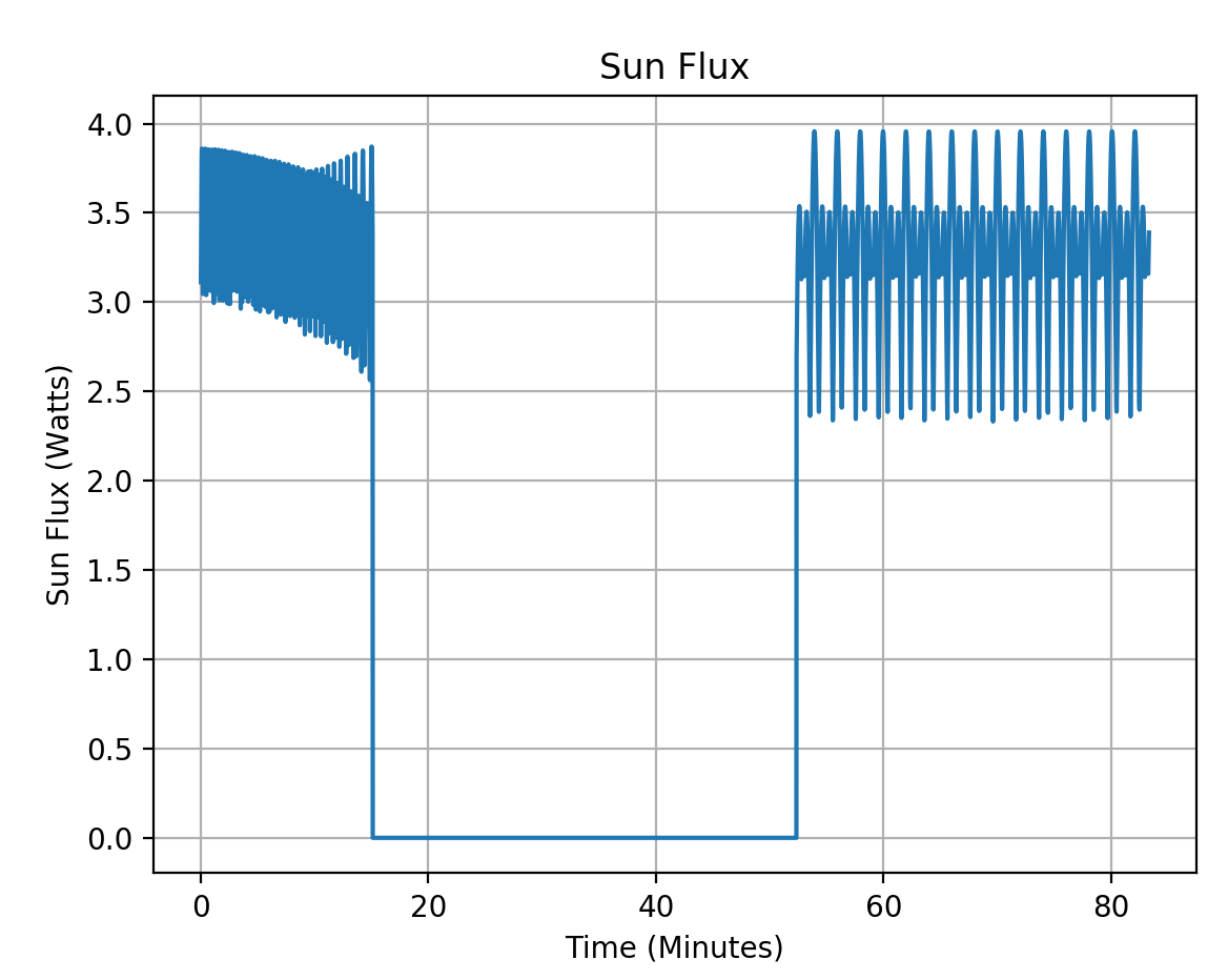
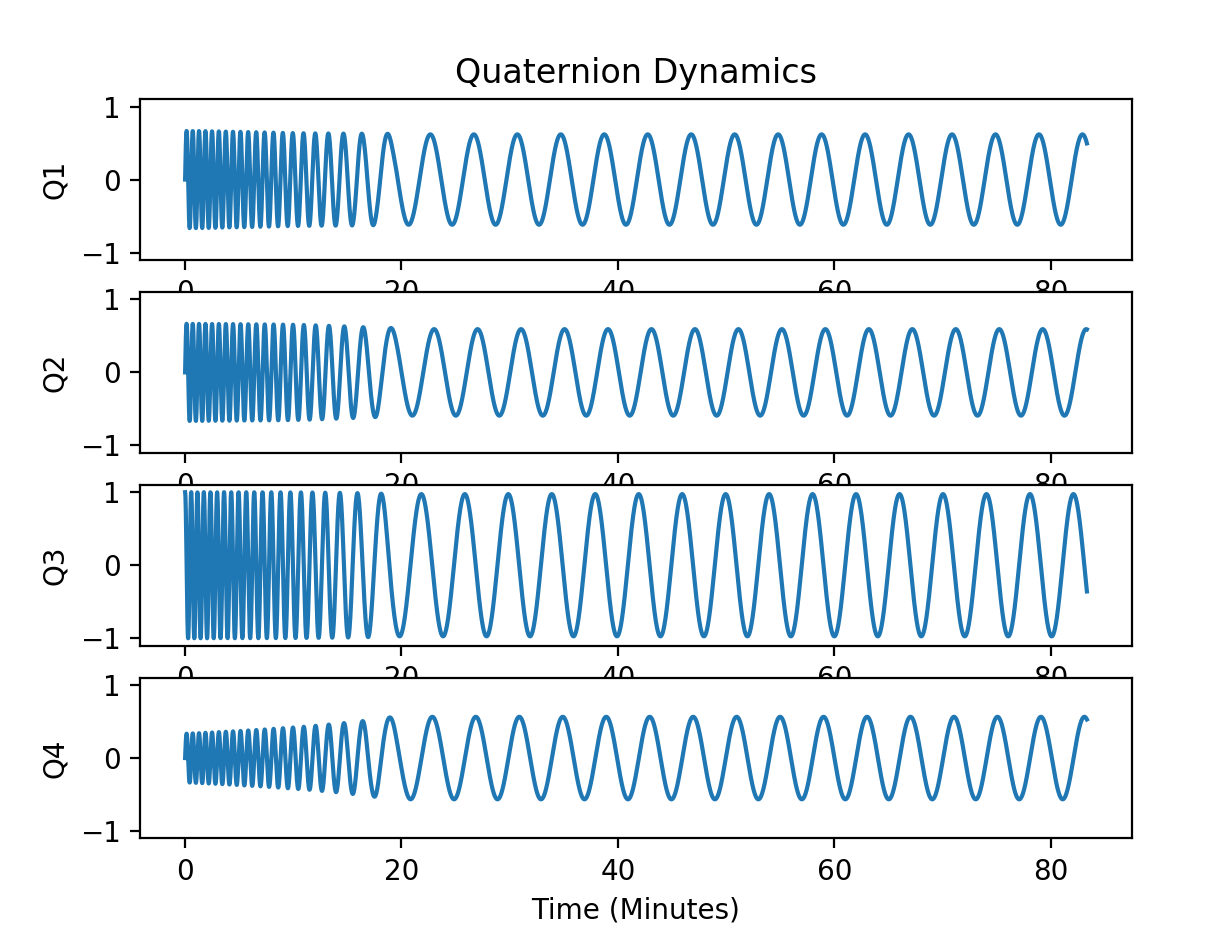
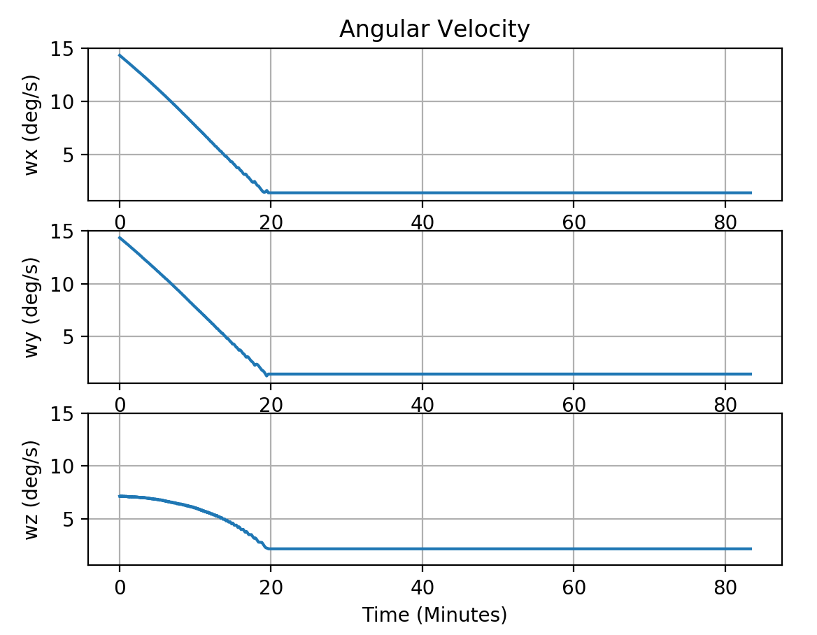
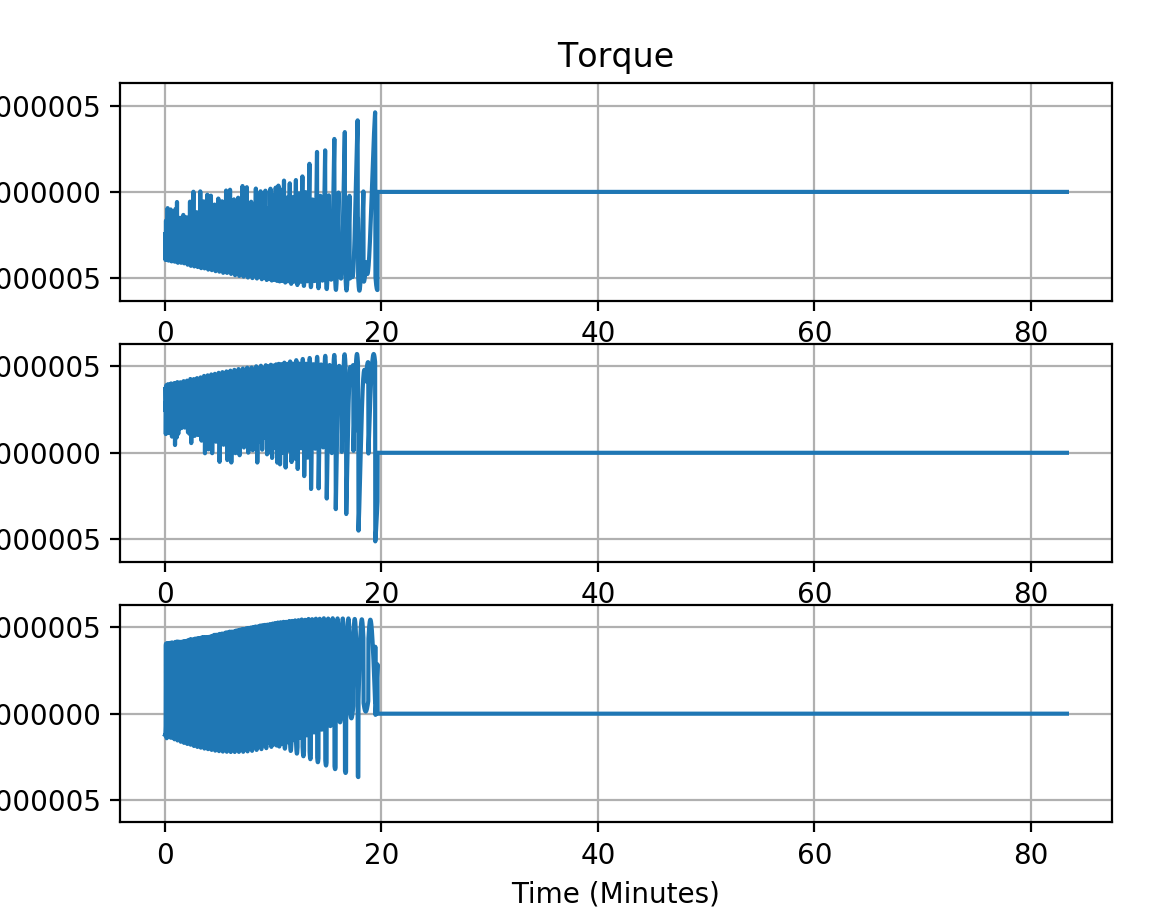
Here are the resulting plots from the simulation. In this specific instance, it was run with initial conditions for angular velocity of . The Orbit given is the ISS orbit, and the initial position is given by a true anomaly of 100 degrees. The spacecraft takes around 20 minutes to detumble below a threshold of 3 degrees per second, after which the magnetorquers are turned off, and angular velocities remain constant in the absence of perturbing forces. The power generation plot goes to zero during the eclipse in the orbit.

Quaternion Dynamics:

Angular Velocities:

Torque Applied:

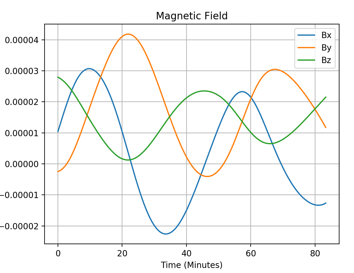
Magnetic Field Over the Orbit

Orbital Position:

Solar Power Generation Throughout Orbit: