Causality

Causal representation learning

• Paper: Towards Causal Representation Learning
• Goal: discover high-level causal variables (a representation (partially) exposing the unknown causal structure, which variables describe the system and their relations) from high-dimensional and low-level observations.

Invariant risk minimization (IRM)

• Paper: Invariant Risk Minimization

• A side point: mixing and shuffling dataset from different environment can discard what information is stable across training environments.

  Shuffling is used to make the distribution of training data and test data similar based on the i.i.d. assumption of machine learning, but when collecting data from different environment (not i.i.d.) and mixing them to receive a big dataset and shuffling them when training, we destroy how the data distribution changes across data sources.

  This side point motivates that each environment should be considered separately.

• IRM principle: To learn invariances across environments, find a data representation such that the optimal classifier on top of that representation matches for all environments.

• Assumption: the data from all the environments share the same underlying structural equation model.

Basic formulation of the problem

• Datasets:
  
• Goal: learn a predictor Y ≈ f(x) to minimize the maximum loss of the predictor in all environments
  

IRM formulation

• Formal goal:
  
  This thought searching for invariance clarifies common induction methods in science.
• Constrained optimization problem:
  The formal goal can be achieved with two steps:
    1: Mind for the data representation Φ to predict well;
    2: Elicit an invariant predictor ω among the useful representations.
  Then, the constrained optimization problem is to minimize empirical risk but subject to invariant predictors, which can be stated as:
  
  As this formulation of IRM is a hard solved bi-leveled optimization problem, then it need to be instantiate into some practical version.
• IRMv1:
  
  In this version, Φ becomes the entire invariant predictor, and ω =1.0 is a scalar and fixed "dummy" classifier. The theoretical process for IRMv1 is stated as follows:

  Step 1: translate IRM into the penalized loss
     
  Step 2: assume ω as a linear-least squares regression and design the penalty
     
     Then, choose a simple penalty based on discrepancy between classifiers of each environment and the optimal one:
     
     However, as the existence of matrix inversion in the explicit solution of ω, this penalty results in a discontinuous case. Therefore, it can be simplified by multiplying both sides to construct a new version:
     
  Step 3: fix the linear classifier ω with an invertible mapping
     Due to the problem of over-parameterization, rewriting the invariant predictor with an invertible mapping Ψ as:
     
     Then, the relaxed version of IRM becomes:
     
  Step 4: set fixed classifier to monitor invariance
     The authors supposed
     
     Then, they proposed theorem 4 as
     
     Proof:
        
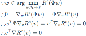
     From theorem 4, the dimension of classifier ω is unspecified and is selected with the dimension of representation Φ. Then, to simplify the problem, ω is set to be fixed scalar 1.0, and the optimization object becomes:
     
  Step 5: extend to general loss
     Using the penalty obtained in Step 2, the general function of loss can be written as:
     
     Proof:
     

Environment inference

Environment inference

• Paper: Environment Inference for Invariant Learning
• Idea: Using a probability distribution q to a soft assignment of environments, which is obtained by capturing the worst-case environments for a fixed classifier

Heterogeneous Risk Minimization

• Paper: Heterogeneous Risk Minimization

The risks of invariant risk minimization

• Paper: The Risks of Invariant Risk Minimization

Information bottleneck for invariant risk minimization (IB-IRM)

• Paper: Invariance Principle Meets Information Bottleneck for Out-of-Distribution Generalization

Bayesian invariant risk minimization (BayesionIRM)

• Paper: Bayesian Invariant Risk Minimization

Sparse invariant risk minimization (SparseIRM)

• Paper: Sparse Invariant Risk Minimization

Problem setting

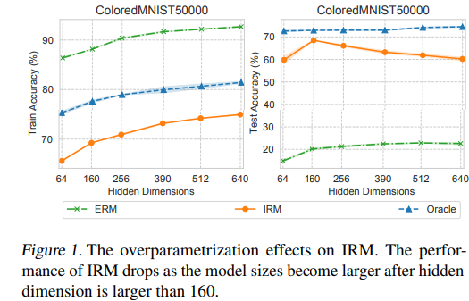
• Problem: IRM performs poorly in the case of over-parameterized deep neural netowrk.
  

  Empirical verification:
  
  Theoretical proof:
     
  In addition, the authors find out that the reason of overfitting is mistakenly using some spurious features.
  
  Theoretical proof:
     

Solution

• Key idea: The authors use sparsity constraint in the training process to make the subnetwork small so that the spurious and random features is prevented from leaking into the subnetwork and the network has to identify and focus on invariant features to achieve smaller loss.
• Sparse invariant risk minimization objective:
  
  where m is a binary mask to perform feature selection, K is used to control the total model size. In practice, m is reparameterized to be a independent Bernoulli random variables and transform the optimization objective as :
  

Structured representation

• Paper: Structure by Architecture: Structured Representations without Regularization

CausalVAE

• Paper: CausalVAE: Structured Causal Disentanglement in Variational Autoencoder

CITRIS

• Paper: CITRIS: Causal Identifiability from Temporal Intervened Sequences
• TRIS: temporal intervened sequences
  Data generated by a latent temporal causal process with causal factors.

iCITRIS

• Paper: iCITRIS: Causal Representation Learning for Instantaneous Temporal Effects
• iTRIS: instantaneous temporal intervened sequences
  Data generated by a latent temporal causal process with causal factors, including causal relations across time steps (i.e. temporal) and within a time step (i.e. instantaneous).

CRP model

• Paper: Time Series Prediction With Events Disturbance Based Causal Representation Learning