Used cars prices dataset analysis - Tornadosky/Cars-price-prediction GitHub Wiki
We use dataset from Kaggle for used car auction price prediction. The dataset contains various features that are required to predict and classify the range of prices of used cars.
import matplotlib
import matplotlib.pyplot as plt
import numpy as np
import pandas as pd
import seaborn as sns
import plotly
from scipy import stats
import warnings
warnings.filterwarnings("ignore")
Libraries for ML
from sklearn import preprocessing
from sklearn.ensemble import RandomForestRegressor
from sklearn.model_selection import train_test_split
from sklearn.tree import DecisionTreeRegressor
data = pd.read_csv('car_prices.csv', on_bad_lines='skip')
print("row number: ", len(data))
print("column number: ", len(data.columns))row number: 558811
column number: 16
data.head(3)| year | make | model | trim | body | transmission | vin | state | condition | odometer | color | interior | seller | mmr | sellingprice | saledate | |
|---|---|---|---|---|---|---|---|---|---|---|---|---|---|---|---|---|
| 0 | 2015 | Kia | Sorento | LX | SUV | automatic | 5xyktca69fg566472 | ca | 5.0 | 16639.0 | white | black | kia motors america, inc | 20500 | 21500 | Tue Dec 16 2014 12:30:00 GMT-0800 (PST) |
| 1 | 2015 | Kia | Sorento | LX | SUV | automatic | 5xyktca69fg561319 | ca | 5.0 | 9393.0 | white | beige | kia motors america, inc | 20800 | 21500 | Tue Dec 16 2014 12:30:00 GMT-0800 (PST) |
| 2 | 2014 | BMW | 3 Series | 328i SULEV | Sedan | automatic | wba3c1c51ek116351 | ca | 4.5 | 1331.0 | gray | black | financial services remarketing (lease) | 31900 | 30000 | Thu Jan 15 2015 04:30:00 GMT-0800 (PST) |
data.info()<class 'pandas.core.frame.DataFrame'>
RangeIndex: 558811 entries, 0 to 558810
Data columns (total 16 columns):
# Column Non-Null Count Dtype
--- ------ -------------- -----
0 year 558811 non-null int64
1 make 548510 non-null object
2 model 548412 non-null object
3 trim 548160 non-null object
4 body 545616 non-null object
5 transmission 493458 non-null object
6 vin 558811 non-null object
7 state 558811 non-null object
8 condition 547017 non-null float64
9 odometer 558717 non-null float64
10 color 558062 non-null object
11 interior 558062 non-null object
12 seller 558811 non-null object
13 mmr 558811 non-null int64
14 sellingprice 558811 non-null int64
15 saledate 558811 non-null object
dtypes: float64(2), int64(3), object(11)
memory usage: 68.2+ MB
print("Most important features relative to selling price:")
corr = data.corr()
corr.sort_values(["sellingprice"], ascending = False, inplace = True)
print(corr.sellingprice)
Most important features relative to selling price:
sellingprice 1.000000
mmr 0.983634
year 0.586488
condition 0.538788
odometer -0.582405
Name: sellingprice, dtype: float64
data.describe()| year | condition | odometer | mmr | sellingprice | |
|---|---|---|---|---|---|
| count | 558811.000000 | 547017.000000 | 558717.000000 | 558811.000000 | 558811.000000 |
| mean | 2010.038696 | 3.424512 | 68323.195797 | 13769.324646 | 13611.262461 |
| std | 3.966812 | 0.949439 | 53397.752933 | 9679.874607 | 9749.656919 |
| min | 1982.000000 | 1.000000 | 1.000000 | 25.000000 | 1.000000 |
| 25% | 2007.000000 | 2.700000 | 28374.000000 | 7100.000000 | 6900.000000 |
| 50% | 2012.000000 | 3.600000 | 52256.000000 | 12250.000000 | 12100.000000 |
| 75% | 2013.000000 | 4.200000 | 99112.000000 | 18300.000000 | 18200.000000 |
| max | 2015.000000 | 5.000000 | 999999.000000 | 182000.000000 | 230000.000000 |
data.isnull().sum()year 0
make 10301
model 10399
trim 10651
body 13195
transmission 65353
vin 0
state 0
condition 11794
odometer 94
color 749
interior 749
seller 0
mmr 0
sellingprice 0
saledate 0
dtype: int64
We don't need columns "seller", "saledate" and "vin" since they don't influence the price. "mmr" though seems to influence the price a lot, but according to it's defenition and correlation it's actually a variable that depends on every other feature. We dropped it too.
data = data.dropna(how='any')
data.drop(columns=['vin', 'seller', 'saledate','mmr'], inplace=True)
Here is what we have as a result:
data.shape(472336, 12)
%matplotlib inline
data.hist(bins=50, figsize=(20,15))
plt.show()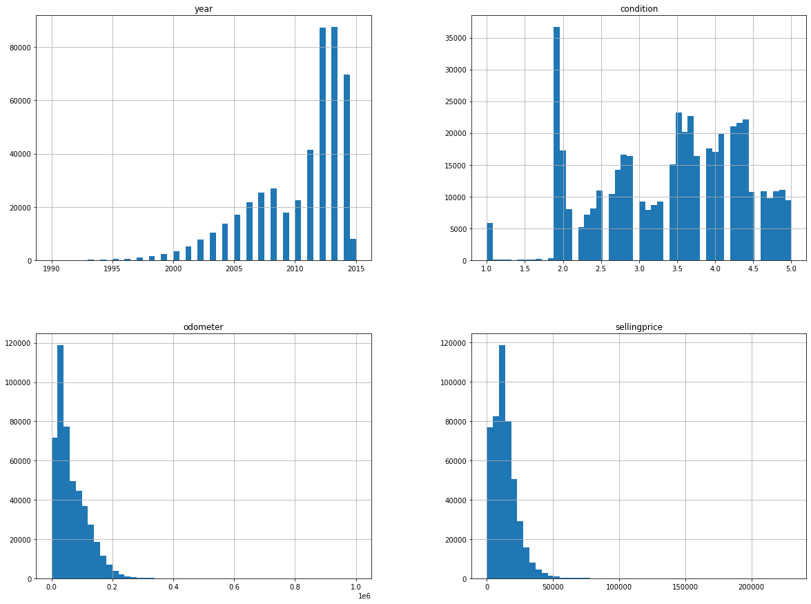
listtrain = data['make']

# prints the missing in listtrain
print("Missing values in first list:", (set(listtrain).difference(listtrain)))
Missing values in first list: set()
There are some values like "SUV" and "suv" in our dataset, so we make all string occurances in lower case.
data['transmission'].replace(['manual', 'automatic'],
                        [0, 1], inplace=True)

prev_unique = len(data['body'].unique())

for col in data.columns:
    if type(data[col][0]) is str:
        data[col] = data[col].apply(lambda x: x.lower())

curr_unique = len(data['body'].unique())

data.head(5)| year | make | model | trim | body | transmission | state | condition | odometer | color | interior | sellingprice | |
|---|---|---|---|---|---|---|---|---|---|---|---|---|
| 0 | 2015 | kia | sorento | lx | suv | 1 | ca | 5.0 | 16639.0 | white | black | 21500 |
| 1 | 2015 | kia | sorento | lx | suv | 1 | ca | 5.0 | 9393.0 | white | beige | 21500 |
| 2 | 2014 | bmw | 3 series | 328i sulev | sedan | 1 | ca | 4.5 | 1331.0 | gray | black | 30000 |
| 3 | 2015 | volvo | s60 | t5 | sedan | 1 | ca | 4.1 | 14282.0 | white | black | 27750 |
| 4 | 2014 | bmw | 6 series gran coupe | 650i | sedan | 1 | ca | 4.3 | 2641.0 | gray | black | 67000 |
print(prev_unique, curr_unique)85 45
data.isnull().sum()year 0
make 0
model 0
trim 0
body 0
transmission 0
state 0
condition 0
odometer 0
color 0
interior 0
sellingprice 0
dtype: int64
data.dtypesyear int64
make object
model object
trim object
body object
transmission int64
state object
condition float64
odometer float64
color object
interior object
sellingprice int64
dtype: object
data.describe()| year | transmission | condition | odometer | sellingprice | |
|---|---|---|---|---|---|
| count | 472336.000000 | 472336.000000 | 472336.000000 | 472336.000000 | 472336.000000 |
| mean | 2010.211045 | 0.965359 | 3.426576 | 66701.070003 | 13690.403670 |
| std | 3.822131 | 0.182868 | 0.943659 | 51939.183430 | 9612.962279 |
| min | 1990.000000 | 0.000000 | 1.000000 | 1.000000 | 1.000000 |
| 25% | 2008.000000 | 1.000000 | 2.700000 | 28137.000000 | 7200.000000 |
| 50% | 2012.000000 | 1.000000 | 3.600000 | 51084.000000 | 12200.000000 |
| 75% | 2013.000000 | 1.000000 | 4.200000 | 96589.000000 | 18200.000000 |
| max | 2015.000000 | 1.000000 | 5.000000 | 999999.000000 | 230000.000000 |
After preprocessing the data, it is analyzed through visual exploration to gather insights about the model that can be applied to the data, understand the diversity in the data and the range of every field.
data.head(3)| year | make | model | trim | body | transmission | state | condition | odometer | color | interior | sellingprice | |
|---|---|---|---|---|---|---|---|---|---|---|---|---|
| 0 | 2015 | kia | sorento | lx | suv | 1 | ca | 5.0 | 16639.0 | white | black | 21500 |
| 1 | 2015 | kia | sorento | lx | suv | 1 | ca | 5.0 | 9393.0 | white | beige | 21500 |
| 2 | 2014 | bmw | 3 series | 328i sulev | sedan | 1 | ca | 4.5 | 1331.0 | gray | black | 30000 |
Now, let's check the Price first.
sns.distplot(data['sellingprice'])

print("Skewness: %f" % data['sellingprice'].skew())
print("Kurtosis: %f" % data['sellingprice'].kurt())
Skewness: 2.003565
Kurtosis: 12.057796
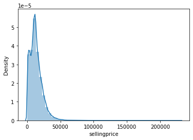
We can observe that the distribution of prices shows a high positive skewness to the left (skew > 1). A kurtosis value of 12 is very high, meaning that there is a profusion of outliers in the dataset.
# applying log transformation
data['sellingprice'] = np.log(data['sellingprice'])
# transformed histogram and normal probability plot
sns.distplot(data['sellingprice'], fit=None);
fig = plt.figure()
res = stats.probplot(data['sellingprice'], plot=plt)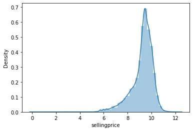
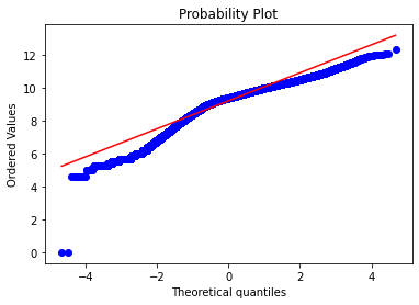
We found that converting the value of sellingprice to Log(sellingprice) might be a good solution to have a more normal visualization of the distribution of the Price, however, this alternative has no major or decisive effect on the results of the train and/ or predict procedure in the next section. Therefore, in order not to complicate matters, we decided to keep the whole processed database up to this step to analyze the parameters' correlations and conduct the modeling in the following section.
To compute the price for vehicles, this platform may compute linear regression model that defines a set of input variables. However, it does not give details as what features can be used for specific type of vehicles for such prediction. We have taken important features for predicting the price of used cars using random forest models.
The author of some jupyter notebook evaluates the performance of several classification methods (logistic regression, SVM, decision tree, Extra Trees, AdaBoost, random forest) to assess the performance on similar dataset. Among all these models, random forest classifier proves to perform the best for their prediction task.
This work uses 11 features ('Cars', 'Location', 'Year', 'Kilometers_Driven', 'Fuel_Type', 'Transmission', 'Owner_Type', 'Mileage', 'Engine', 'Power', 'Seats') to perform the classification task after removal of irrelevant features from the dataset which gives an accuracy of 96.2% on the test data. We also use Kaggle data-set to perform prediction of used-car prices.
A. Data preparation & Model Parameters
In this Notebook, we do not discuss in deep about the Models' parameters, we just applied the standard or refer to previous recommendations. Let's copy the database.
import copy
df_train=copy.deepcopy(data)

cols=np.array(data.columns[data.dtypes != object])
for i in df_train.columns:
    if i not in cols:
        df_train[i]=df_train[i].map(str)
df_train.drop(columns=cols,inplace=True)df_train.head(10)| make | model | trim | body | state | color | interior | |
|---|---|---|---|---|---|---|---|
| 0 | kia | sorento | lx | suv | ca | white | black |
| 1 | kia | sorento | lx | suv | ca | white | beige |
| 2 | bmw | 3 series | 328i sulev | sedan | ca | gray | black |
| 3 | volvo | s60 | t5 | sedan | ca | white | black |
| 4 | bmw | 6 series gran coupe | 650i | sedan | ca | gray | black |
| 5 | nissan | altima | 2.5 s | sedan | ca | gray | black |
| 6 | bmw | m5 | base | sedan | ca | black | black |
| 7 | chevrolet | cruze | 1lt | sedan | ca | black | black |
| 8 | audi | a4 | 2.0t premium plus quattro | sedan | ca | white | black |
| 9 | chevrolet | camaro | lt | convertible | ca | red | black |
And then, coding the categorical parameters using LabelEncoder.
from sklearn.preprocessing import LabelEncoder
from collections import defaultdict

# build dictionary function
cols = np.array(data.columns[data.dtypes != object])
d = defaultdict(LabelEncoder)

# only for categorical columns apply dictionary by calling fit_transform
df_train = df_train.apply(lambda x: d[x.name].fit_transform(x))
df_train[cols] = data[cols]df_train.head(10)| make | model | trim | body | state | color | interior | year | transmission | condition | odometer | sellingprice | |
|---|---|---|---|---|---|---|---|---|---|---|---|---|
| 0 | 24 | 637 | 873 | 39 | 2 | 17 | 1 | 2015 | 1 | 5.0 | 16639.0 | 9.975808 |
| 1 | 24 | 637 | 873 | 39 | 2 | 17 | 0 | 2015 | 1 | 5.0 | 9393.0 | 9.975808 |
| 2 | 4 | 8 | 255 | 36 | 2 | 7 | 1 | 2014 | 1 | 4.5 | 1331.0 | 10.308953 |
| 3 | 52 | 582 | 1243 | 36 | 2 | 17 | 1 | 2015 | 1 | 4.1 | 14282.0 | 10.230991 |
| 4 | 4 | 33 | 338 | 36 | 2 | 7 | 1 | 2014 | 1 | 4.3 | 2641.0 | 11.112448 |
| 5 | 36 | 64 | 104 | 36 | 2 | 7 | 1 | 2015 | 1 | 1.0 | 5554.0 | 9.296518 |
| 6 | 4 | 413 | 389 | 36 | 2 | 1 | 1 | 2014 | 1 | 3.4 | 14943.0 | 11.082143 |
| 7 | 7 | 177 | 47 | 36 | 2 | 1 | 1 | 2014 | 1 | 2.0 | 28617.0 | 9.190138 |
| 8 | 2 | 46 | 71 | 36 | 2 | 17 | 1 | 2014 | 1 | 4.2 | 9557.0 | 10.381273 |
| 9 | 7 | 118 | 846 | 5 | 2 | 14 | 1 | 2014 | 1 | 3.0 | 4809.0 | 9.769956 |
print("Most important features relative to selling price:")
corr = df_train.corr()
corr.sort_values(["sellingprice"], ascending = False, inplace = True)
print(corr.sellingprice)
Most important features relative to selling price:
sellingprice 1.000000
year 0.776455
condition 0.624522
transmission 0.070842
trim 0.047761
color 0.030101
state -0.020057
model -0.022356
make -0.035849
body -0.072775
interior -0.168183
odometer -0.717036
Name: sellingprice, dtype: float64
We split our dataset into training, testing data with a 70:30 split ratio. The splitting was done by picking at random which results in a balance between the training data and testing data amongst the whole dataset. This is done to avoid overfitting and enhance generalization.
ftrain = ['year', 'make', 'model','trim', 'body', 'transmission',
          'state', 'condition', 'odometer', 'color', 'interior', 'sellingprice']

def Definedata():
    # define dataset
    data2 = df_train[ftrain]
    X = data2.drop(columns=['sellingprice']).values
    y0 = data2['sellingprice'].values
    lab_enc = preprocessing.LabelEncoder()
    y = lab_enc.fit_transform(y0)
return X, y%%time
from sklearn.ensemble import RandomForestRegressor
model = RandomForestRegressor()
X, y = Definedata()
X_train, X_test, y_train, y_test = train_test_split(X, y, test_size = 0.25)
model.fit(X_train,y_train)
model.score(X_test, y_test)0.9487117477394104