Stanford Sparse Autoencoder - SummerBigData/MattRepo GitHub Wiki
In this exercise we implemented a sparse autoencoder algorithm to show that edges are a nice representation of natural images. We were supplied with 10 (512, 512) images of different landscapes. Here is what some of the images looked like in greyscale.
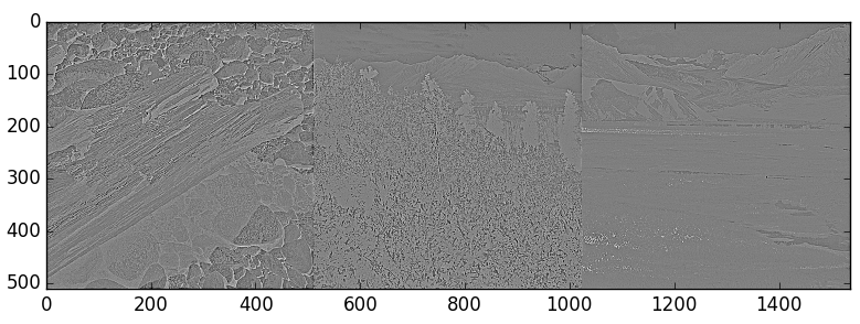
We needed to create a (10000, 64) array, where each row represents a random (8, 8) patch from a random picture. Then, we trained our autoencoder on this data and looked at how well it reconstructed each patch. We needed to change the range of our inputs because the pixel values ranged from -1 to 1, and we needed them to be from 0 to 1 instead since our sigmoid function outputs values on a range from 0 to 1. Also, we visualized what input image would maximally activate one of the nodes in our hidden layer. We also set up our backprop and cost function to use linear regression this time. Our weights for computing a2 (hidden layer) was of size (25, 64) and the bias layer was created separately and was of size (25, 1). Our weights for computing a3 (output layer) was of size (64, 25) and the bias layer was, again, created separately and was of size (64, 1). The separation of our weights and bias layers made setting up our backpropagation function a bit easier. We ran our code for different lambda values ranging from 1e-3 to 1e-6. Our beta values stayed at 3 and our sparse parameter was set to 0.01 for all tests. Here is what in the input and outputs look like side by side:
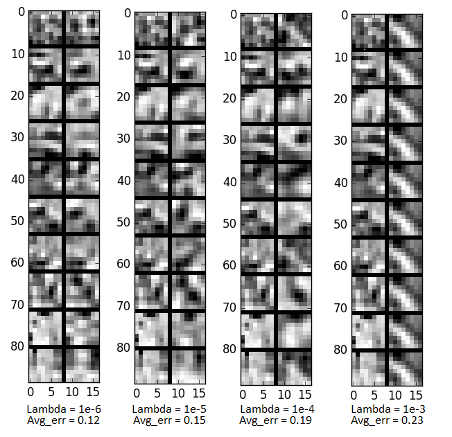
We calculated the average error of each pixel using this equation

Now for visualizing the input that would maximally activate one of the nodes in our hidden layer. This was done by using the equation

where x was assumed to be normalized bectween 0 and 1 (which it is).
Here are the visualizations for different lambdas:
Lambda = 1e-6
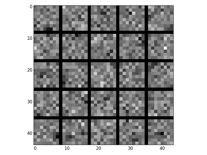
Lambda = 1e-5
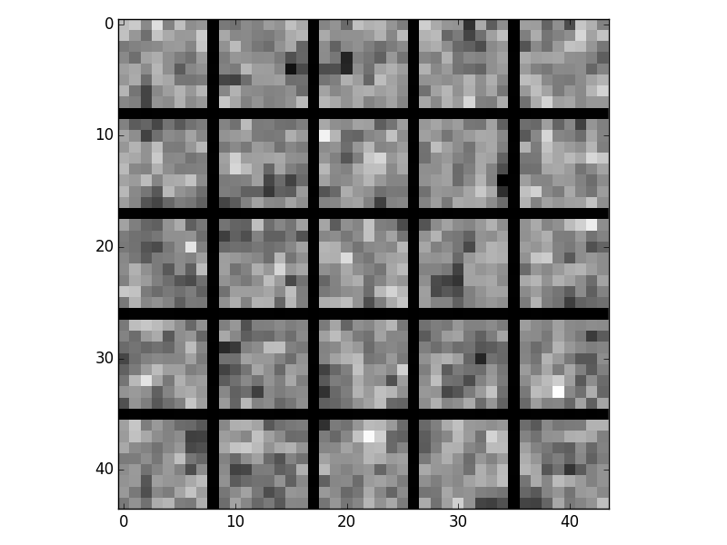
Lambda = 1e-4
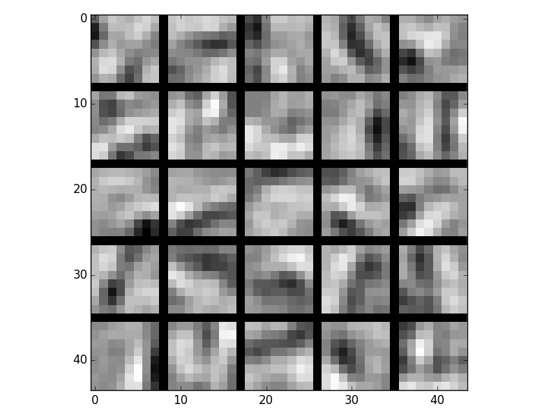
Lambda = 1e-3
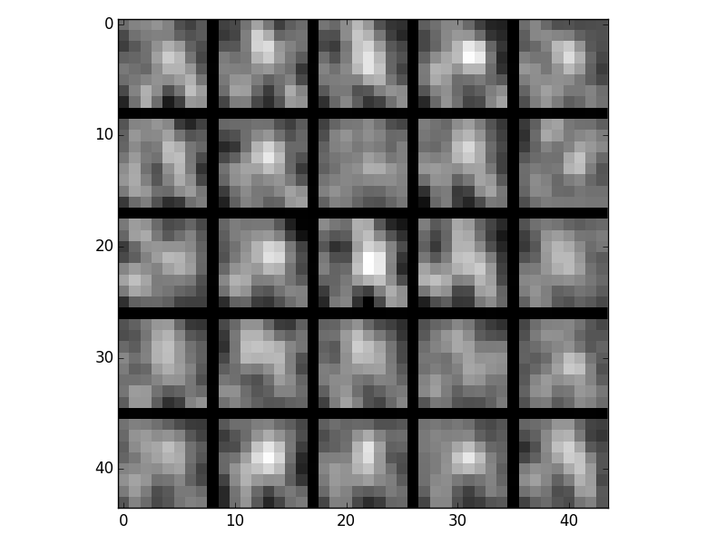
The images with lambda = 1e-4 have noticable edges.