Stanford Exercise 3 - SummerBigData/MattRepo GitHub Wiki

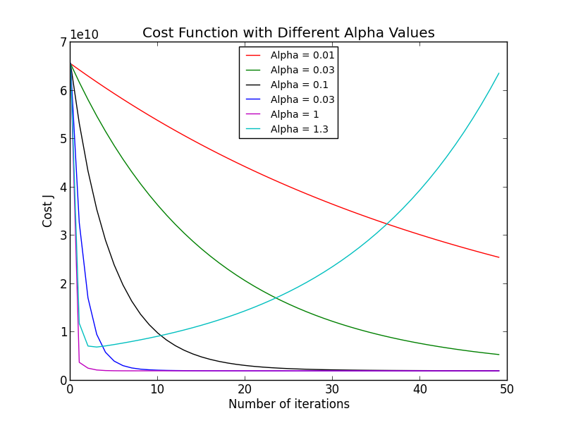
In this exercise we looked at mulivariate linear regression using both gradient descent and normal equations. We were provided a training set that consisted of housing prices in Portland, Oregon. The y values are the prices of the house and the x values consist of both the living area and the number of bedrooms. There were a total of 47 training examples. First, gradient descent was used to to find the best learning rate for our cost function J(theta). Due to how large the the living areas could be we had to normalize our x values so our gradient descent equation would require less iterations to converge. The graph below shows us the different values of alpha that were used.

The cost function converged the fastest when alpha was equal to one. So, this will be the value we use to find our theta values since it will converge faster than any other values. It should be noted that an alpha value of 1.3 ended up diverging, so the cut off for when alpha is too big is between 1 and 1.3. After some tests the value seems to be around 1.28 when our cost function diverges. Using the alpha value we picked our final values for theta0, theta1, and theta2 are 340413, 109448, and -6578.35 respectively. We then predicted the price for a 1650-square-foot house with 3 bedrooms to be 293081 dollars.

Next we used the normal equations to find our theta values. This method did not require us to normalize our x values, nor use any alpha values. From using this method our final values for theta0, theta1, and theta2 are 89597.9, 139.211, and -8738.02 respectively. Again, we predicted the price for a 1650-square-foot house with 3 bedrooms to be 293081 dollars.