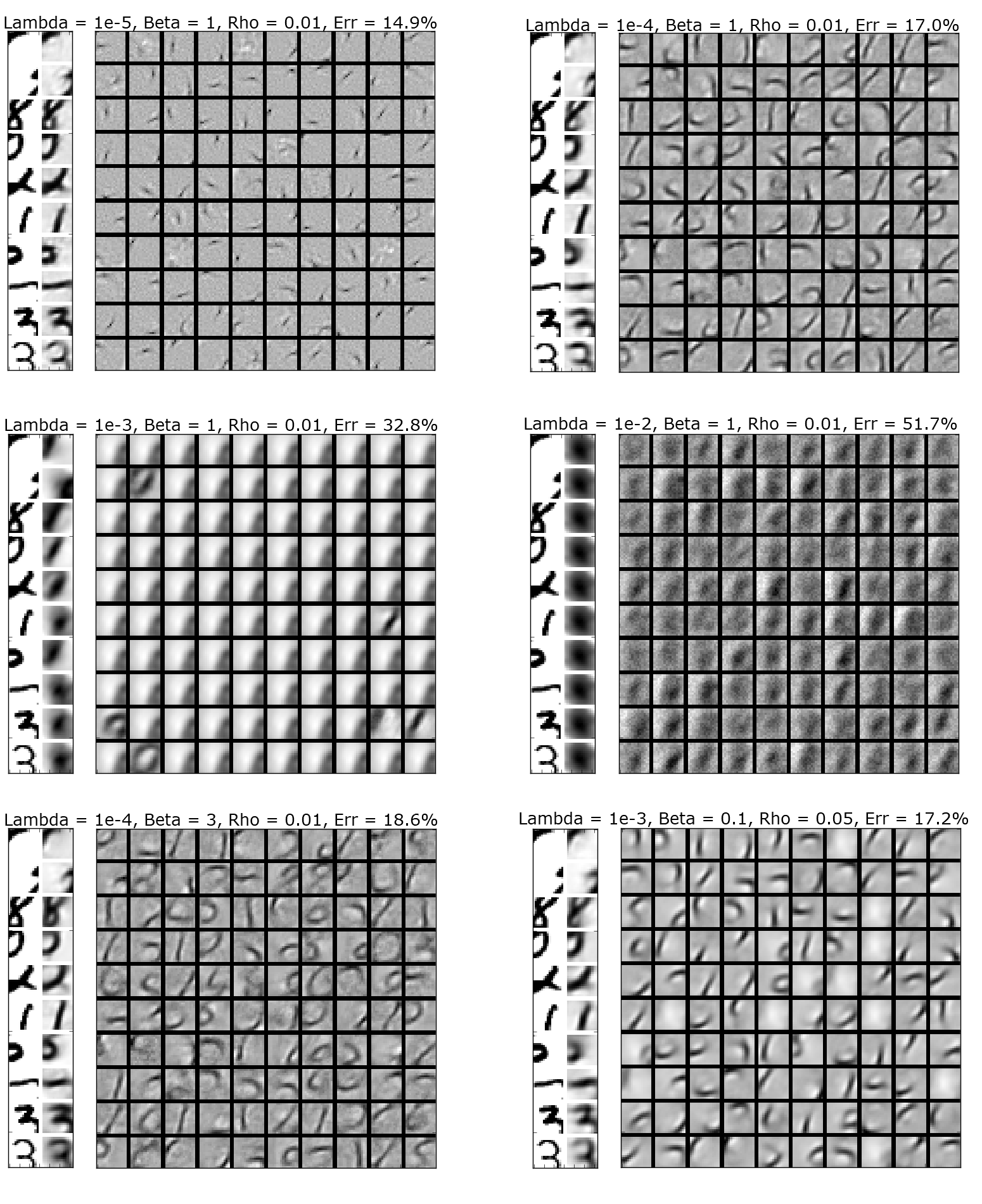
This exercise was done similar to the one involving the STL-10 subset of images, but now we are using the MNIST data set. This means instead of having images in RGB we just have greyscale, simplifying our sparse autoencoder and convolution. First we set up a function that gave use 10k (15, 15) patches from random MNIST digit images that would be used in our sparse autoencoder. We chose (15, 15) to avoid having any patches that showed only white space. In our sparse autoencoder we ran multiple tests with different lambda values with a hidden layer of size 100, here are what some of the max activations looked like.

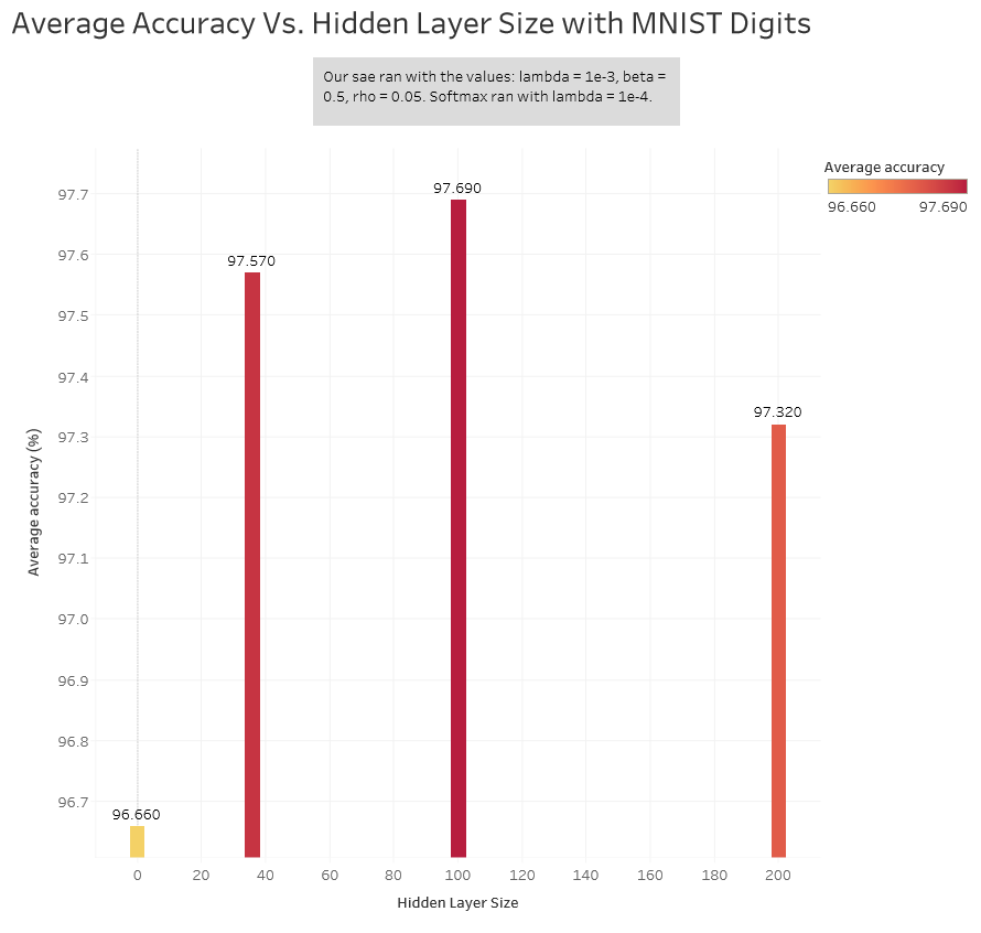
The image on the bottom right was with Suren's parameters. The max activations are less grainy and look more like pen strokes, so we chose those parameters to work with. We then went on to convolving and pooling (mean pooling) the features that were learned from these patches with the full 60k training set and 10k test set. The final size would be (2, 2) features for both the training and test set. We chose to reduce the size of the features to (2, 2) since (7, 7) was too large and when trying to reshape with this size we ran into memory problems (had 16gb allocated). We ran our softmax classifier with different hidden layer sizes to see what the best size would be when training on our pooled features. The hidden layer was computed using logistic regression while the output layer used softmax regression. Here are the different accuracies.

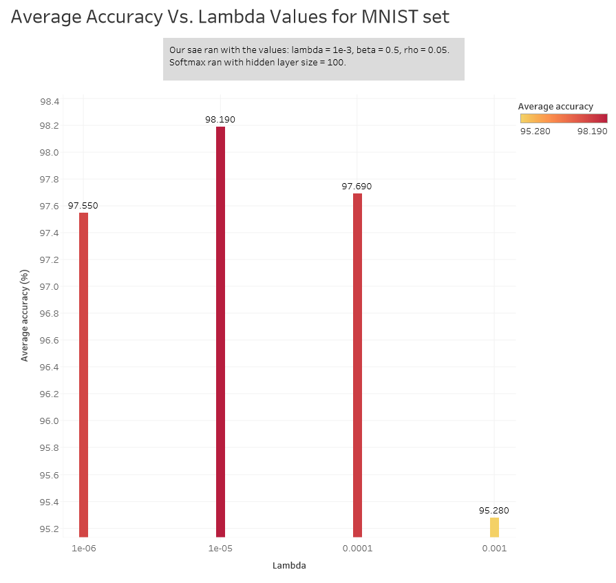
We chose to use a hidden layer size of 100 since that gave us the best results and tried different lambda values on it. Here are the average accuracies.

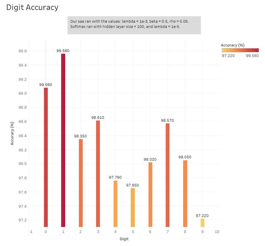
A lambda of 1e-5 gave us the best average accuracy. Here are the individual accuracies for each digit with this value of lambda.

Instructions

Since we didn't follow the instructions given in the exercise here are the steps we took to complete this exercise.

1. Extracted 10k (15, 15) patches from random images in the MNIST dataset.

Code used

2. Ran the patches through our sparse autoencoder using a hidden layer size of 100 (Code was set up in a previous exercise). The best values we used were Lambda = 1e-3, Beta = 0.5, Rho = 0.05.

Code used

3. Loaded the features into a python code that would call a function for convolution and a function for pooling (Code was done in a previous exercise with the STL-10 images). Main differences are having a 100 hidden layer size instead of 400, grabbing the MNIST data instead of STL-10 images, and not dealing with whitening or subtracting the mean off of anything.

4. Numbers 5 and 6 were done in batches of 20 features until all 100 were convolved and pooled.

5. Convolved features. The code from STL-10 to MNIST is different. You do not need to do any whitening or mean subtracting and you can remove the for loop used for the three different colors since the MNIST dataset is greyscale.

Used on STL-10

Used on MNIST

6. Pooled features (Used the same code from previous exercise on STL-10). Dimension of our pooling region was 7, so after pooling our features were (2, 2).

7. Used softmax classifier (Done in previous STL-10 exercise). Main difference is obtaining MNIST data instead of STL-10 data. Optimal lambda value was 1e-5.