Coursera Exercise 3 - SummerBigData/MattRepo GitHub Wiki

In this exercise we used one-vs-all logistic regression along with neural networks to recognize hand written digits. These digits ranged from 0 to 9. We were provided a matlab file that contained an X matrix and a y matrix. The X matrix consisted of a (5000, 400) matrix where each row represented a number. Images can be put together into a (20, 20) grid to show what they are. Here are a couple of examples:

Here's a list of the numbers in order:

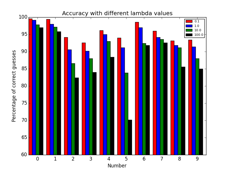
The y matrix was a column vector that had the numbers 1-10 in it indicating what number each corresponding row in our X matrix represented. The number 10 was used for 0 since matlab doesn't start its indices at 0. We then set up a vectorized cost function, cost function gradient, and sigmoid function. We implemented regularizing for the cost function and the cost function gradient. We then proceeded to use one-vs-all classification. We trained a classifier for each digit in our dataset. We did this by setting the digit we wanted to train equal to 1 and the rest equal to 0 in our y array and did this for each digit. We then minimized our cost function and stored the computed thetas for each digit. We took those thetas and our X matrix and plugged it into the sigmoid function to get the probabilities of what each digit was. Afterwards we looked to see how accurate our program was at identifying the numbers given. Here is a graph of how accurate our program is based on different lambdas:

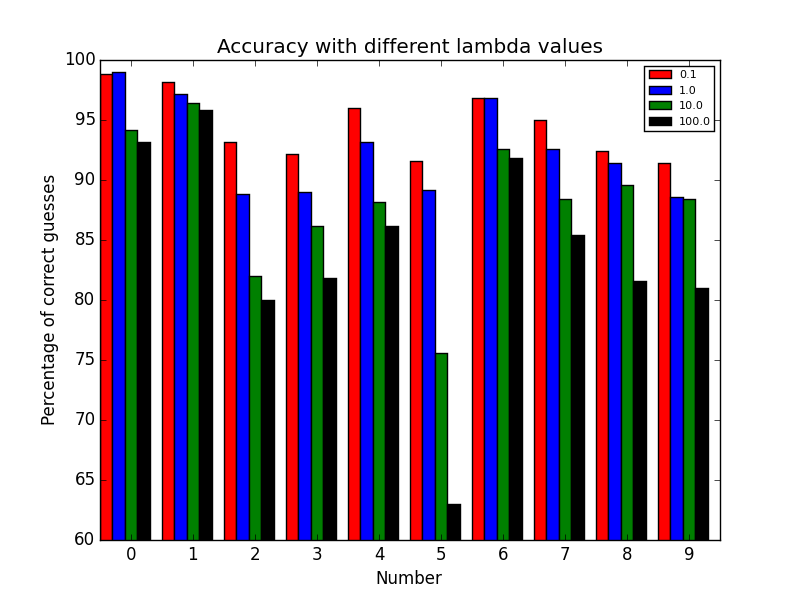
The CG method was used to minimize our cost function. We can see as our lambda got larger the accuracy dicreased. So we are not over-fitting as much as lambda increases. Here is a bar graph when the BFGS method was used to minimize our cost function:

On average it looks like the accuracy of our program was worse using this method.

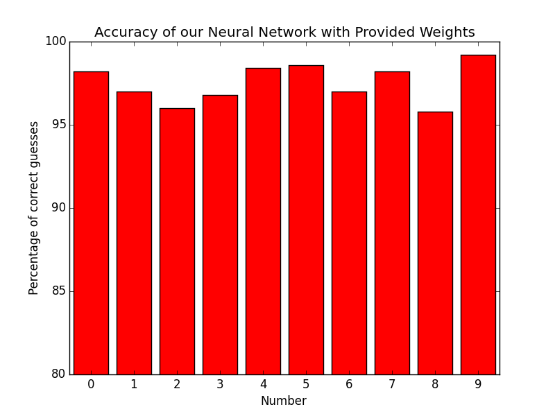
We then implemented a neural network using the weights that were supplied to us. We were given a (25, 401) theta matrix for the first use of our sigmoid equation, and a (10, 26) theta matrix for our second use of our sigmoid equation. We used feedforward propogation to find our predictions from each time we used our sigmoid function. Our accuracy is as follows:

0: 98.2% correct

1: 97.0% correct

2: 96.0% correct

3: 96.8% correct

4: 98.4% correct

5: 98.6% correct

6: 97.0% correct

7: 98.2% correct

8: 95.8% correct

9: 99.2% correct

Here is a bar graph to accompany these percentages:

We also decided to take a peak into the hidden layer and see what our numbers looked like inside. Here is an image of one set of numbers that ranges, in order, from 0-9.