Jason Fleming [email protected] v2.0, June 2014, Seahorse Coastal Consulting:

The ADCIRC Surge Guidance System (ASGS) is a software system for generating storm surge and wave guidance from ADCIRC + SWAN in real time on high resolution grids. The ASGS constructs meteorological forcing from a parametric wind / pressure model using storm parameters extracted from National Hurricane Center (NHC) Forecast Advisories. During nor'easters or for day-to-day generation of tidal forecasts and other results, the system uses gridded wind and pressure fields (e.g., NCEP’s NAM model) as input forcing. In both cases, hydrologically-driven river forecast data from NSSL can also be used to account for the effects of precipitation and upland river flooding.

Warning: Some people treat their ASGS installation as a fragile thing to be protected If you can't unceremoniously dispatch your ASGS installation to /dev/null and start from scratch with out fuss, then you're doing it wrong or ASGS needs to support whatever customization you're needing. Please let us know. You should not be hacking ASGS to get it working for you.

Over the years of using ASGS operationally, the "system" has become easier to re-install than debug. This approach works well when a storm is approaching and minutes matter. Operators do not need to be wasting valuable time debugging their ASGS installation or treating it like a precious, fragile thing.

Instead, it is encouraged to simply reinstall ASGS on a system if things start acting strange. When new versions of ASGS are released, it is likewise often recommended that you just create a brand new environment. You are free to keep the old one around, of course, but the value of it is with the configuration files.

If you find yourself modifying ASGS scripts, thus locking yourself into a particular directory and "version". DON'T. Please find out how you can create a clean and repeatable environment from scratch. If ASGS' installation infrastructure can't handle your situation, let us know. It's highly likely someone experienced with managing ASGS installations is able to make a valuable suggestion or even extend ASGS in some way to unfetter you from an old customized ASGS, which many tend to regard over time as some black box that they are afraid to sneeze at.

Finally, if you can't reinstall ASGS and get your stuff working in just a few steps, then you're at risk of getting tied down. Please let us know and we can help make ASGS bend to you, repeatedly and predictably.

Related to our admonission about treating your ASGS installation as special, is the subject of this section. ASGS configuration files should be only as complex as necessary. In the sections below, there is discussion of some environmental settings (e.g., PERL5LIB). Please take note that many of these variables are managed by the ASGS Shell Environment, and it is a red flag if an operator finds themselves setting them without good reason. If you find you're in a situation that seems to warrant this extreme action, please let us know.

An overview of the modular structure of the ASGS is shown in Figure 1. The figure indicates the separation of System components into the following categories:

• reference information (in purple), which specify the system configuration and physical parameter data used in the simulation;

• dynamic input data (in red) that varies in time and must be downloaded from external data sources for every forecast cycle;

• input file production (in green), which implements the system behavior specified by the Operator in the system configuration files; and

• output visualization, publication, and interaction (in blue) for use by clients and end users.

• The overall structure of the ASGS divides the various features into their own modules. The configuration and static physical data that are common to all simulation runs are shown at the top in purple, the dynamic data acquisition modules are shown in red, the internal data processing and input file generation are shown in green, and output modules are shown in blue at the bottom. Arrows are conceptual and indicate data flow.

[caption="Figure 1. "] image::http://www.seahorsecoastal.com/figures/asgs_structure_color.png[align="center",width=500] These categories and associated modules will be described in greater detail below.

The reference information includes a dynamic specification of system behavior in the configuration file as well as static physical data, embodied in the simulation input files ADCIRC. The system configuration consists of a single file, and all of the features and behavior of the various components can be controlled from this single configuration file. This file is used to activate or deactivate the various types of physical forcing, including tropical cyclone meteorology, ordinary meteorology, wave simulation and coupling, tides, and river flow input.

It is also used to specify a wide variety of other settings, including (for example) the type of computer that the system is running on, the number of processors to use in parallel execution, the name of the ADCIRC mesh file for the domain of interest, the number of storms in an ensemble and their characteristics, the types of output products to generate, the email addresses of officials that should be notified when results are ready, and many others.

The simulation input files represent a purely static set of physical data that are used in the simulations. These data include the ADCIRC mesh (domain discretization), the bathymetry and topography of the domain, the spatially varying Manning's n value, and the directional wind roughness lengths and canopy effects derived from land cover data.

The static data also include the tidal constituents to be included (if any), convergence controls and solution parameters for SWAN and ADCIRC, the names and locations of point recording stations for location-specific output data, and other data related to the internal procedures of the simulation codes.

The system is capable of downloading and preparing dynamic meteorological data from two sources: the National Hurricane Center's (NHC) Forecast/Advisories, and the National Centers for Environmental Prediction's (NCEP) North American Mesoscale (NAM) model, depending on the data source selected by the Operator. Furthermore, the system has a module for downloading river boundary flow data from the National Severe Storms Laboratory and preparing it for use in ADCIRC.

For tropical cyclone events, the NHC Forecast/Advisories are downloaded by the system as soon as they are issued, and the relevant storm parameters (including storm positions. maximum wind speeds, and isotach radii) are parsed into a format that ADCIRC can use to generate wind fields using an internal asymmetric vortex model. For ordinary meteorology, including nor'easters and other systems, the system downloads regularly gridded meteorological fields from the NAM model from the NCEP ftp site. The gridded meteorological fields are extracted from the grib2 format that NCEP uses, reformatted and written to OWI formatted files that ADCIRC reads.

Once meteorological data have been obtained, the system downloads the latest river flow data from the National Severe Storms Laboratory (NSSL) ftp site. These data are in a file format that ADCIRC can read natively, and are set up to correspond to a particular ADCIRC mesh. The module that downloads these data must splice a series of these files together to match the date and time range implied by the meteorological data that have already been obtained.

Once the Operator has created a configuration file and assembled the static physical input data for a particular instance of the system and initiates startup, the system reads its configuration file and tries to determine its state: whether it is starting “hot” with a simulation that is already in progress, or “cold”, where a new ADCIRC or ADCIRC+SWAN simulation must be started from scratch (see Figure 2).

It also makes a determination about the state of its input files; specifically, whether they have already been decomposed for parallel execution. If the system must start from a “cold” state, it creates input files and executes a hindcast simulation to warm up the simulation and prepare it for the cyclical nowcast/forecast production phase (described below). Accordingly, this hindcast run is set so that it writes a hotstart file at the very end to represent the state of the warmed-up simulation.

In addition, if the input files have not been prepared for parallel execution, the system decomposes them for the specified number of processors. If the hindcast and/or decomposition tasks are required, they must only be performed once at the start of the system's execution (processes that occur at most one time during an execution of the system are shown in blue in Figure 2).

.The overview of the logic of the ASGS divides the one-time start up process for an initially "cold" simulation state in blue, with the bulk of the time being spent in the nowcast/forecast cycle, indicated by green. [caption="Figure 2. "] image::http://www.seahorsecoastal.com/figures/asgs_overview_color.png[align="center"] /

The nowcast occurs next if the simulation state is already "hot" when the system starts up, or if the system has already performed the decomposition and warm up phases. The first step in the nowcast is to determine if there are new meterological data available, by contacting the associated external website or ftp site, checking the timestamps that are available there, and comparing them with the current simulation time. If there are data available that are more recent than the current simulation time, a new cycle is deemed to have begun, and those data are downloaded. The system downloads the data it requires to cover the time period between its current simulation time and the most recent data that are available files that are available. After the meteorological data have been acquired, river data are acquired in the same way, if they have been specified.

Once the external data have been acquired, the input files for the ADCIRC simulation code (and the SWAN simulation code if wave forcing has been specified by the Operator in the system configuration file) are constructed using the time range of the meteorological forcing files and the various configuration parameters in the system configuration file. This includes tidal boundary conditions, output file formats and frequency of production of output files, and locations for point recording of output for comparison with tide gages or meteorological data collection equipment. The nowcast control file(s) for ADCIRC and SWAN are set to write a hotstart file at the end of the simulation for use in starting the forecast, as well as a future nowcast. The last file written during the nowcast phase is the queue script that will be used to submit the job to the high performance computer's queueing system.

Once the nowcast is complete, the system acquires the data required for one or more forecasts. These data will already be present in the case of a tropical cyclone, since the NHC forecast/advisory has already been parsed. For NAM forcing, the NAM forecast data are downloaded from NCEP and converted to OWI using the same technique as described for the nowcast. If river flux forcing was specified, the river flux data are downloaded and formatted in a similar manner to the nowcast. The control files are constructed to cover the time period implied by the forecast meteorological data, but are not set to write a hotstart file at the end. When the forecast is complete, the system executes post processing (described in the next section) and archives the data as required.

These forecast process described above is applied to each member of the forecast ensemble until all ensemble members have been completed, at which point the system goes back to looking for new meteorological data for its next nowcast.

The application of meteorological forcing presented a challenge for operational storm surge forecasts because of the need for timely availability of high resolution input data. The most accurate data-assimilated meteorological fields from the HWind project were only available for nowcast and hindcast times, and even then were not available until several hours had passed after a corresponding hurricane advisory had been issued from the NHC. In addition, regularly gridded meteorological data from models such as the North American Mesoscale (NAM) model had a relatively coarse grid resolution in comparison to the unstructured ADCIRC mesh (12km grid resolution vs 30m minimum mesh resolution).

In contrast, parametric wind models produce comparable storm surge in many cases (Houston et al, 1999; Mattocks et al 2006). They also had the following advantages: (1) they require a comparatively tiny quantity of input data; (2) they could be coded as fast subroutines that run in-process; (3) they could provide wind stress and barometric pressure at arbitrary locations.

As a result of the advantages of parametric wind models, the Holland model (Holland, 1980) was selected as the basis of the wind speed and pressure field. Modifications and additions were made to the published model to account for the dynamic changes in the hurricane parameters along the hurricane's track, as well as its adaptation to the data available from the NHC advisory, as described below. This modified model was referred to as the Dynamic Asymmetric Holland Model.

The hurricane advisory contained at least the following information for each forecast increment: date, time, latitude and longitude of the center of the storm, and maximum observed wind speed at 10m with a 1 minute sampling interval. In addition, the distance to isotachs at various wind speeds were sometimes provided in one or more storm quadrants.

The vortex model was set up to operate in a two step process. The first step was the use of isotach data from the forecast/advisory to calculate a representative radius to maximum winds (Rmax) in each of the four storm quadrants, for each forecast increment, before the actual ADCIRC run. The second step was to interpolate the resulting Rmax for all nodes at each time step of the simulation, to determine the wind velocity throughout the domain at each time step.

The first step was performed in a pre-processing program for all the data from a particular forecast/advisory, before the ADCIRC run began. This design provided visibility to the Rmax values that ADCIRC would use, and gave the Operator the capability to modify the input values for experimentation.

The representative Rmax values were determined for each quadrant and forecast increment by subtracting the translation speed of the storm from the maximum wind speed, and converting both the translation-reduced maximum wind speed and the highest isotach wind speed in that quadrant into the equivalent wind speeds at the top of the atmospheric boundary layer. These wind speeds and the distance to the highest isotach in that quadrant were then substituted into the gradient wind equation. The gradient wind equation was then solved for the Rmax in that quadrant using Brent's method, or if that failed numerically, a brute force marching algorithm.

The pre-processing program then appended the resulting Rmax values to the meterological input file for use in the actual ADCIRC simulation.

The second step occured during the execution of ADCIRC. For each time step in the simulation, the central pressure, latitude and longitude of the storm center, and radii to maximum winds were interpolated in time to reflect the simulation time relative to the forecast increments provided by the National Hurricane Center. The translation speed from the most recent forecast increment was used to reduce the time-interpolateed maximum wind speed. The time-interpolated maximum wind radii were interpolated in space using a cubic spline; the relevant value of Rmax at each node was determined from the cubic spline curve. Finally, the Holland(1980) model was used to determine the nodal wind velocity using the spline-interpolated Rmax, the translation-reduced value of the maximum wind speed, and a Holland B whose value was calculated and then limited to the range of 1.0 to 2.5.

After the computation of the nodal wind velocities at the top of the atmospheric boundary layer, the magnitudes were reduced to corresponding values at 10m, and then reduced again from the 1 minute averaging used by the National Hurricane Center to 10 minute averaging required by ADCIRC. A "damped" translational velocity was vectorially added to the nodal wind velocities, where the damping was proportional to the distance from the radius to maximum winds.

Finally, the wind vectors were rotated toward the center of the storm by an angle that depended on the distance from the center: the rotation angle was ten degrees between the center and the radius to maximum winds; it was twenty five degrees beyond 1.2 times the radius to maximum winds; and the rotation angle was linearly interpolated from the ten degree value at Rmax and the 25 degree value at 1.2 times Rmax.

.The hurricane vortex model embedded in ADCIRC was used to generate wind velocity and barometric pressure at each timestep of the simulation using isotach radii (depicted at top left) extracted from the National Hurricane Center Forecast/Advisories. A streamline visualization of the surface wind speeds is shown at top right, and the profiles of wind speed in each quadrant and barometric pressure in each quadrant are shown at bottom left and bottom right respectively.

[caption="Figure 3. "] image::http://www.seahorsecoastal.com/figures/irene25_vortex_analysis.png[align="center",width=700]

The production of human-comprehensible output is arguably the most important step in the entire process. Clients must be notified that new results are available; and they must be able to get to and use the results in a way that is intuitive for them. As there is more than type of end user or client, there is more than one approach to producing useful output: (a) publication of raw data; (b) production and publication of static images, non-interactive animations, and results files in domain specific formats; and (c) elucidation via interactive visualization through a web application.

Publication of raw results is the most basic step for post processing, and an OpenDAP server is recommended for use in publication of raw data in NetCDF format to clients and end users. An OpenDAP server provides a web interface to the data, making it easy for users to simply click on a link to the graphics or data file they wish to download, either for the latest run or for any previous simulation run. Technologies such as NCTOOLBOX are available for sophisticated end users to apply their own analyses to the raw data, producing the output they require locally. Once the data have been posted to the OpenDAP server, the system sends an email to a list of email addresses as specified in the system configuration file to notify them that new results are available.

The next level of presentation is in-situ post processing, that is, running non-interactive graphics generation programs in the high performance computing environment to generate static images, non-interactive animations, and reformatted versions of results in specialty fomats. These techniques are all in currently place, and have the advantage of not requiring voluminous quantities of data to be moved to an external server for post processing. For example, the system produces GIS shape files, JPEG images and non-interactive animations of maximum inundation as well as Google Earth (kmz) images of maximum inundation, all with in-situ post processing. These output products are then published to the OpenDAP server to make them available to clients. The disadvantage of in-situ processing is the lack of interactivity.

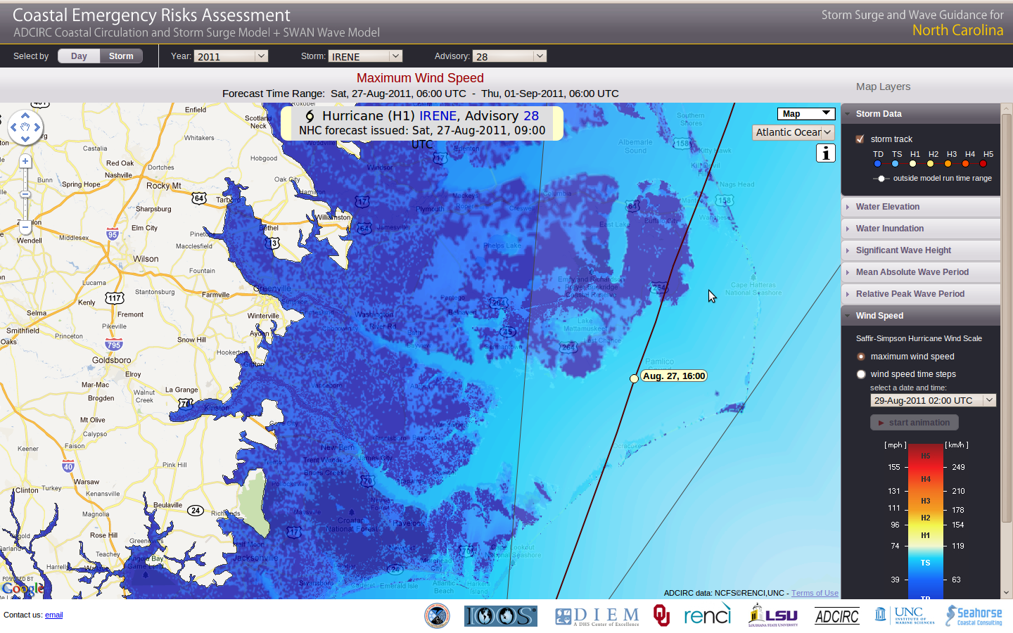
The most effective type of presentation is the use of an interactive web visualization application to elucidate results and provide interactivity. For this level, the Coastal Emergency Risks Assessment (CERA) interactive web application was deployed and used to provide an interactive interface that served the needs of non-technical as well as experienced clients.

.The CERA interactive web visualization of maximum wind speed for Irene advisory 25 in real time shows the swath of maximum wind speeds along the consensus forecast track. The storm name and year dropdown menus are visible at the top of the interface, with accordion type menus for each type of output data along the right side. [caption="Figure 4. "]

image::http://www.seahorsecoastal.com/figures/irene25_maxwind.png[align="center",width=700]

The CERA application integrates visualization ADCIRC and ADCIRC+SWAN results with Google Maps to provide the context for the results as well as practical features such as panning and the ability to zoom in more closely at various areas of interest to see greater resolution and detail. The application organizes results by storm and advisory (for tropical cyclone results) or by cycle (for NCEP NAM results). It presents these options concisely via dropdown boxes across the top of its interface.

.The maximum significant wave height from SWAN for Irene advisory 23 in real time shows the tremendous open water wave heights that were being generated by the storm at its peak intensity, as well as the size of the waves that were actually impinging on the coastline. [caption="Figure 5. "]

image::http://www.seahorsecoastal.com/figures/irene23_maxwaveheight.png[align="center",width=700]

/images/irene25_maxwaveheight.png

The right side of the interface is an accordion-type menu that presents the various types of data that are available, including water surface elevation, inundation, significant wave height, wave period, and wind speed. For each type of data, the application is able to present a zoomable image of the maximum values that occurred over the course of the forecast (e.g., high water marks) as well as a zoomable, stoppable animation that illustrates the evolution of the data through time.

.The maximum water surface elevation from Irene advisory 28 in real time provided emergency managers with high water mark data that indicated the hardest hit areas that required immediate attention. [caption="Figure 6. "]

image::http://www.seahorsecoastal.com/figures/irene28_maxele.png[align="center",width=700]

Furthermore, the interface allowed the user to click on any point of the storm track to view the data that are relevant to the time when the storm was at that point in the track. It is also capable of presenting the nodes of the underlying ADCIRC mesh, and displaying detailed summary information for any particular node the user selects.

.This close-up of the maximum wind speed from Irene advisory 28 in real time shows the consensus forecast track of the storm as well as the local wind speeds. The dark blue colors show the results of the land use data described previously, and the resulting surface roughness lengths that knock down the force of the wind. The directionality of the roughness lengths can be seen by carefully examining the wind shadows on the Neuse and Pamlico rivers. [caption="Figure 7. "] image::http://www.seahorsecoastal.com/figures/irene28_maxwind_closeup.png[align="center",width=700]

The CERA application works by using the OpenDAP server as a staging area for raw data. The CERA application received notification email from the NCFS that new results were published to the OpenDAP server in NetCDF format. It would then download these data as well as some summary information about the type of forecast run that produced the data. It generated visualizations via production of image tiles at progressively finer scales, thus providing the user with the ability to zoom in and examine results in greater detail. These image tiles were then stored on the web server where the data were published, and sent to web clients as required by the user interaction with the web application and its menu system.

The ASGS is set up for a particular modeling situation using a configuration file. Information in the ASGS configuration file is generally restricted to parameters that are determined by the scientific and logistical choices of the Operator. In contrast, configuration that is particular to a the underlying HPC platform is covered in the ASGS Developers Guide, and platform-specific configuration is generally contained within the ASGS itself, rather than an external configuration file.

The ASGS continually re-reads its configuration file; it is first read upon startup, and then once before every nowcast and forecast. This gives the ASGS a degree of dynamic configurability.

One unique aspect of the ASGS configuration file is that it is also a shell script. As a result, the configuration parameters are actually (bash) shell script variables, and are set as such. The use of a shell script as a configuration file also comes in handy if the desired configuration requires some logic, or the use of simple arrays; examples of both will be provided in the following sections.

On the other hand, one of the side effects of the use of a shell script as a configuration file is that it is dangerous to comment out the variables in the configuration file, or to set them equal to "". This causes the associateed value to be "missing" in the list of arguments to various subroutines within the ASGS, which moves all the other command line arguments up one place, causing many issues.

In order to avoid these issues, the solution is to leave unneeded configuration parameters alone, rather than commenting them out or setting them to "". If the values are not useful, or not needed, the ASGS will generally deal with them gracefully. There aren't any features or behavior of the ASGS that are triggered by the mere presence of a particular configuration parameter in the configuration file. Parameters can be set to the word "null" for lack of any appropriate value; examples of this are provided below.

Each of the following sections details the parameters that are present in the configuration file. The sections start with a brief description of the section, followed by a snippet from a real configuration file. The definitions of the parameters in that section are then provided in detail. The definitions may be followed by a discussion of how the configuration parameters are used by the ASGS.

In an actual ASGS configuration file, the configuration parameters can be provided in any order.

Fundamental configuration includes the name of the ASGS instance, resources required, and the type and timing of system startup.

INSTANCENAME=2 # "name" of this ASGS process COLDSTARTDATE=2012042500 # calendar year month day hour YYYYMMDDHH24 HOTORCOLD=coldstart # "hotstart" or "coldstart" LASTSUBDIR=null # path to previous execution (if HOTORCOLD=hotstart) HINDCASTLENGTH=45.0 # length of initial hindcast, from cold (days) REINITIALIZESWAN=no # used to bounce the wave solution

Definitions

• INSTANCENAME

The instance name can be any string; a single digit integer is used in practice. The instance name is helpful when multiple instances of the ASGS are running on the same machine. It can also be used to label results, to indicate which instance (among several on a particular machine) generated the results.

• COLDSTARTDATE

This date corresponds to ADCIRC time=0; it is used in many different ways by the ASGS, but the principal uses are as follows: (a) determination of nodal factors and equilibrium arguments for tidal forcing; (b) determination of the relationship between the current simulation state (along with the hotstart time) and the available input data.

• HOTORCOLD

This parameter can either be set to 'coldstart' or 'hotstart'. When set to 'coldstart', the ASGS will start by performing a hindcast as as described in the previous section. If it is set to 'hotstart', the ASGS will hotstart the simulation using the hotstart file found in the location indicated by the 'LASTSUBDIR' parameter described below.

• LASTSUBDIR

The full path to the last good nowcast (or hindcast) subdirectory must be provided here if the ASGS is meant to start by resuming a simulation that is already in progress.

For example, if the full path to the hotstart file is /srv/asgs99999/initialize/hindcast/fort.67, then the LASTSUBDIR parameter should be set to /srv/asgs99999/initialize.

If the full path to the hotstart file is /srv/asgs88888/2012010100/nowcast/fort.67, the LASTSUBDIR parameter should be set to /srv/asgs88888/2012010100. In other words, the ASGS wants to find either a hindcast or nowcast subdirectory under the LASTSUBDIR directory. The ASGS always sets ADCIRC to write a fort.67 file (not a fort.68 file), and only on a hindcast or nowcast, never on a forecast. If the HOTORCOLD parameter is set to coldstart, this parameter can be set to null.

• HINDCASTLENGTH

The length of the hindcast is only used by the ASGS if it actually has to perform the hindcast; that is, if the ASGS is supposed to coldstart ADCIRC.

• REINITIALIZESWAN

The reinitialization of SWAN parameter can be set to "yes" to re-coldstart SWAN (not ADCIRC) at the start of the nowcast in case the SWAN solution develops issues but the ADCIRC solution has not. Set this back to "no" when the SWAN solution has normalized, or else ASGS will continue to re-coldstart SWAN on every nowcast.

The physical forcing that is applied via ADCIRC is controlled via the following configuration parameters; these parameters are each set to +on+ or +off+.

BACKGROUNDMET=on # NAM download/forcing TIDEFAC=on # tide factor recalc TROPICALCYCLONE=off # tropical cyclone forcing WAVES=on # wave forcing VARFLUX=on # variable river flux forcing

Definitions

• BACKGROUNDMET

Set to background meteorology to +on+ to activate meteorological forcing with data from the North American Meoscale (NAM) model from the National Centers for Environmental Prediction (NCEP). Data are acquired from the NCEP ftp site. If this is turned on, then TROPICALCYCLONE must be set to off (i.e., these types of forcing are mutually exclusive).

• TIDEFAC

Set the tidal factor parameter to +on+ to activate tidal forcing, which causes the nodal factors and equilibrium arguments to be recalculated for every simulation run.

• TROPICALCYCLONE

The tropical cyclone forcing parameter should be set to on to activate meteorological forcing with one of the vortex models that are embedded in ADCIRC. This requires forecast/advisory data from the National Hurricane Center (NHC) as input. Data may be acquired from the NHC web and ftp sites, or may be retrieved from the local file system, as described in the Tropical Cyclone section below. If this is turned on, then BACKGROUNDMET should be turned off (i.e., these types of forcing are mutually exclusive).

• WAVES

The coupling of SWAN to ADCIRC is activated by setting this parameter to on. Because SWAN simulates wind-driven waves, either BACKGROUNDMET or TROPICALCYCLONE must be turned on for the parameter to have any effect.

• VARFLUX

The variable flux parameter is used to activate aperiodic river boundary forcing, and will cause the ASGS to look to an external ftp site for ADCIRC fort.20 files and use that data to construct ADCIRC fort.20 files that are appropriate for the simulation run that it is constructing.

The computational resources available to the ASGS will dictate many of the parameter settings in this section, and these parameter settings are interdependent, as described below.

PPN=8 NCPU=179 # number of compute CPUs for all simulations NUMWRITERS=1 # defacto standard number of global writers is 1 NCPUCAPACITY=360 # total CPUs available to this ASGS instance CYCLETIMELIMIT=05:00:00 # deadline for submitting forecast ensemble

Note: Total number of CPUs per simulations will be NCPU + NUMWRITERS. This total should divide evenly into NCPUCAPACITY. The number of compute nodes is determined by how many compute nodes it'll take to spread NCPU+NUMWRITERS at PPN. Sometimes the full capacity of a computer node is under-utilized in order to dedicate more memory per process, but this is a rare situation and usually part of research or benchmarking activities.

Definitions

• NCPU

The number of CPUs that should be used for all simulations, including hindcast, nowcasts, and each forecast ensemble member.

• PPN

The number of processors per node is a parameter that is only required by certain HPC platforms, and even on those platforms it is generally a static parameter set in asgs_main.sh. It is only supplied in the configuration file if it has to be changed depending on the circumstances of the simulation.

• NUMWRITERS

If dedicated writer processors are to be used in the simulation, the number of dedicated writers is set here. When submitting a compute job, the ASGS will request a number of processors equal to 'NCPU+NUMWRITERS'. If dedicated writers are not to be used, set this value to +0+.

• NCPUCAPACITY

The total number of CPUs available to this instance of the ASGS is specified in the NCPUCAPACITY parameter. If this number is greater than NCPU, the ASGS will be able to submit multiple forecast ensemble members for simultaneous execution. If this number is the same as NCPU, only one compute job will be submitted at a time.

• CYCLETIMELIMIT

The CYCLETIMELIMIT gives the ASGS a deadline to submit all its forecast ensemble member jobs (in hours:minutes:seconds after the current nowcast/forecast cycle was started. This comes into play if there are so many compute jobs or they are executing so slowly that the next forecast cycle is about to start while the ASGS still has jobs to submit from the previous cycle. For example, if the forecast ensemble contains 10 members, and only 5 of them have been submitted to the queue when the CYCLETIMELIMIT (e.g., 5 hours) has passed, the ASGS will refrain from submitting any more. Instead, it will allow the jobs it has already submitted to complete and post process while it starts looking for data to start the next forecast cycle.

Warning: If you are setting these in your ASGS configuration file, it is a red flag. They should only be adjusted if you are familiar with ASGS, the platform and the mesh/ADCIRC scenerios you are running.

HINDCASTWALLTIME="24:00:00" # hindcast wall clock time
ADCPREPWALLTIME="00:15:00"  # adcprep wall clock time, including partmesh
NOWCASTWALLTIME="05:00:00"  # longest nowcast wall clock time
FORECASTWALLTIME="05:00:00" # forecast wall clock time
QUEUENAME=batch             # default queue name on this machine
SERQUEUE=batch              # default queue name (for serial jobs)
TIMESTEPSIZE=0.5            # adcirc time step size (seconds)
SWANDT=1200                 # swan time step size (seconds)

Definitions

• TIMESTEPSIZE

The time step size (in seconds) is used to set the time step on ADCIRC simulations. A shorter time step generally means that the required wall clock time will be longer, all other things being equal.

This tends to be set as part of the mesh defaults.

• SWANDT

The SWAN time step (in seconds) is used to set the time step for SWAN. It should be evenly divisible by the ADCIRC time step size. A shorter timestep generally means a longer wall clock time requirement.

This tends to be set as part of the mesh defaults.

• HINDCASTWALLTIME

The estimated time required to complete the hindcast, whose length (in simulated days) is specified by the 'HINDCASTLENGTH' parameter.

This tends to be set as part of the mesh defaults.

• ADCPREPWALLTIME

The estimated time required to run adcprep, for the longest expected adcprep job type (i.e., partmesh, prepall, prep15).

This tends to be set as part of the mesh defaults.

• NOWCASTWALLTIME

The estimated time required to run a nowcast, taking into account the fact that a nowcast simulation time period may be longer than the typical intercycle simulation time (typically 6 hours) if previous nowcasts have been missed for some reason.

This tends to be set as part of the mesh defaults.

• FORECASTWALLTIME

The estimated time required to run a single member of the forecast ensemble, for the ensemble member with the longest forecast length.

This tends to be set as part of the mesh defaults.

• QUEUENAME

The name of the queue for parallel computational jobs; this is only present in the configuration file if it varies according to the circumstances of the simulation.

This tends to be set as part of the platform defaults.

• SERQUEUE

The name of the queue for serial (single processor) computational jobs, like adcprep; this is only present in the configuration file if the choice of queue varies according to the circumstances of the simulation.

This tends to be set as part of the platform defaults.

The estimates of wall clock time are required because of the need to fill in the estimated wall clock time of the job in the associated queue script when jobs are submitted. Wall clock times are in the format HH:MM:SS, with a leading zero if the number of hours is a single digit.

On computational plaforms where ASGS does not have access to a dedicated queue and is unable to give its jobs special priority over other jobs, the estimated wall clock times should be as small as possible while ensuring that there is enough cushion so that the job is very likely to finish in the estimated time. This is because longer estimated wall clock times generally result in longer waits in a shared queue, with subsequent delays in the production of results.

However, as bad as it is to wait in the queue, it is even worse to have a job killed by the queueing system for exceeding the estimated wall clock limit ... especially if the job was nearly complete at the time it was killed by the system.

In general, an accurate estimate of the wall clock time requires experience with the underlying compute platform as well as the mesh and input files in question. There are many factors that affect wall clock time: number of nodes in the mesh, time step sizes, number of CPUs, implicit vs explicit solution mode in ADCIRC, scalability of the underlying hardware, use of dedicated writer processes, presence or absence of swan coupling, and the type of output files that are being written as well as their frequency of output.

For this particular HPC plaform, there are two queues: a shared queue called "batch" and a high priority queue called "armycore". The platform requires that the number of processors per node be specified, but this parameter depends on the queue to which the job was submitted.

In order to be able to dynamically switch an instance of the ASGS from a low priority queue to a higher priority queue on this platform (for example, if a tropical cyclone is suddenly deemed to be a sufficient threat), the Operator need only change the 'QUEUENAME' from +batch+ to +armycore+, and script takes care of the other settings. The ASGS then propagates the changes in the queuename, the number of processors per node, and the overall number of CPUs requested into the queue scripts that it submits.

Although the overall number of requested CPUs would change in this scenario, the number of compute CPUs would not. Changing the number of compute CPUs dynamically is also possible, unless ADCIRC is set to produce subdomain hotstart files, or wave coupling has been activated. This is because SWAN always produces subdomain hotstart files, which make it difficult to dynamically change the number of compute CPUs, since the SWAN hotstart files would have to be recomposed into a fulldomain SWAN hotstart file, and then redecomposed into the right number of subdomain hotstart files for the new number of CPUs.

During real time operation, the ASGS contacts external sites over the network to acquire the data it needs for its next nowcast/forecast cycle. The configurability of this contact allows the Operator to create mock sites for testing purposes, as well as keep up with changes in the structure of external data sites.

BACKGROUNDMET=OFF                # must be OFF 
TROPCICALCYCLONE=ON              # must be ON
  STORM=03                       # storm number, e.g. 05=ernesto in 2006
  YEAR=2023                      # year of the storm
TRIGGER=rss                      # either "ftp" or "rss"

# defaults (not required unless different)
#RSSSITE=www.nhc.noaa.gov         # site information for retrieving advisories
#FTPSITE=ftp.nhc.noaa.gov         # hindcast/nowcast ATCF formatted files
#FDIR=/atcf/afst                  # forecast dir on nhc ftp site
#HDIR=/atcf/btk                   # hindcast dir on nhc ftp site

Definitions

• STORM

The storm parameter is the two digit storm number assigned by the National Hurricane Center. The name of storm can change, e.g., TD TWELVE can become HU KATRINA, but the number never changes (still 12 in that example). The NHC names data files according to the storm number, not its name.

• YEAR

The four digit year is also used by the NHC to name data files that are relevant to a particular tropical cyclone.

• TRIGGER

The trigger parameter tells the ASGS where to look for new advisories. When set to rss or rssembedded, the ASGS looks at the advisory number in an RSS feed (i.e., an index-at.xml file); when the number changes, a new advisory is deemed to have been issued. In the past, the ASGS always followed a link in the RSS feed to a website with the text of the new forecast/advisory. However, starting with the 2012 season, the NHC has also started embedding the text of the forecast/advisory directly in the xml of their RSS feed. In addition, they sometimes don't update the link to the new forecast/advisory page when they update the advisory number; this issue caused 2 stale advisories to be fed to the ASGS at the start of the 2012 season (1 during Alberto and 1 during Beryl). As a result, the ASGS can now be configured to pull the text of the forecast/advisory directly from the RSS feed, rather than following the embedded link. This feature is activated by setting TRIGGER=rssembedded. In order to configure the ASGS to follow the RSS feed's link to the text of the forecast/advisory, Operators should set TRIGGER=rss. In the past, it was also possible to set the TRIGGER to ftp, causing the ASGS to look for a changed forecast file on the NHC ftp site. As a result of a variety of issues associated with getting forecast/advisory data in ATCF format from the NHC ftp site, TRIGGER should not be set to ftp for tropical cyclone events.

• RSSSITE

The Really Simple Syndication (RSS) site is the website where the ASGS should look for the index-at.xml (the "at" indicates that it is the feed for the Atlantic basin). If RSSSITE is set to filesystem, then FDIR must be set to the full path to the index-at.xml (RSS feed) file on the local filesystem.

• FTPSITE

If FTPSITE is set to filesystem, then HDIR must be set to the path to the bal.dat (ATCF-formatted) hindcast/nowcast data file.

• FDIR

The forecast directory is the path to the index-at.xml on the website where advisories are being issued if RSSSITE is a website. If RSSSITE is set to filesystem, then the forecast directory should be set to the full path to the index-at.xml file on the local filesystem.

• HDIR

The hindcast directory is the path to the bal<STORM><YEAR>.dat file containing the hindcast/nowcast data for the storm <STORM> of year <YEAR> on the ftp site FTPSITE. If FTPSITE is set to filesystem then the hindcast directory should be set to the full path to the bal<STORM><YEAR>.dat file on the local filesystem.

New for the 2012 season, the ASGS can now be configured to load tc hindcast files and/or forecast/advisory files directly from the local filesystem, instead of downloading them from remote web and ftp sites.

This feature is useful for testing, and for production on platforms that do not support direct download of external files. It is activated by setting FTPSITE to filesystem and/or setting RSSSITE to filesystem in the ASGS configuration file. The FTPSITE and RSSSITE configuration parameters are completely independent of each other.

If the RSSSITE is set to filesystem and TRIGGER rss, then the ASGS will load the index-at.xml from the designated location on the local file system and parse out the link to the text of the forecast advisory. If it is a link to a website, it will follow the link to the website.

However, if the forecast/advisory is also on the local filesystem, the <link> tag in the RSS xml should be populated with the full path and file name of the corresponding forecast/advisory text file.

When TRIGGER is set to rssembedded, the ASGS still looks at the advisory number in the RSS feed to determine when a new advisory has been issued, but instead of following a hyperlink, it pulls the text of the forecast/advisory from the RSS feed itself.

When TRIGGER is set to ftp, the ASGS will look for an ATCF-formatted file called al<stormnumber><year>.fst, and compare the content of that file to the last one it downloaded. When the content changes, a new advisory is deemed to have been issued.

The problems with setting TRIGGER to ftp include the following: (a) the ATCF-formatted file does not contain the advisory number; (b) the NHC sometimes issues intermediate advisories simply to update nowcast information, which will look to the ASGS like a new advisory; (c) the file can contain typos which do not affect the ASGS but the typo will be corrected by NHC, causing the ASGS to think a new advisory has been issued.

On the other hand, the ASGS still uses ftp to get the ATCF-formatted BEST track files (that is, the hindcast/nowcast information); it now also has the option of looking to the local filesystem instead of a remote ftp site.

Since TRIGGER=ftp is not used, FDIR is only used by the ASGS when RSSSITE=filesystem, to find the RSS feed (index-at.xml) on the local file system.

BACKGROUNDMET=ON                     # must be ON
  FORECASTCYCLE="00,12"              # in UTC (Z), possible times: 00, 06, 12, 18
TROPICALCYCLONE=OFF
# ... rest of TC's variables are ignored

# defaults (not required unless different)
#BACKSITE=ftp.ncep.noaa.gov          # NAM forecast data from NCEP
#BACKDIR=/pub/data/nccf/com/nam/prod # contains the nam.yyyymmdd files
#FORECASTLENGTH=84                   # hours of NAM forecast to run (max 84)
#PTFILE=ptFile_oneEighth.txt         # the lat/lons for the OWI background met
#ALTNAMDIR="/projects/ncfs/data/asgs5463","/projects/ncfs/data/asgs14174"

Definitions

• FORECASTCYCLE

The forecast cycle parameter tells the ASGS which NAM cycles to run a forecast for, and which NAM cycles it should just nowcast. It will always download forecast files for every cycle in any case. Set this to "00,06,12,18" to run the forecast for all NAM cycles. Set this to +none+ to only run nowcasts (i.e., if forecasting should be turned off).

• BACKSITE

The background meteorological ftp site is the location where the ASGS should look for background meteorological data.

• BACKDIR

The background meteorological directory is the location on BACKSITE where the directories containing NAM output files in grib2 format are located (directory naming convention is nam.yyyymmdd).

• FORECASTLENGTH

Number of hours to forecast; default value is the total length of the NAM forecast (84 hours or 3.5 days).

• PTFILE

The point file contains a list of lat/lon points that the NAM data should be reprojected to during the conversion from grib2 format and Lambert Conformal projection to OWI (ascii text) format and geographic projection. The utility input/ptFile_gen.pl is provided with the ASGS to aid in generating or regenerating files of this type.

• ALTNAMDIR

These local directories are alternate locations for searching for NAM input data on the local filesystem, in case old data cannot be found on the NCEP ftp site. When looking for nowcast files, the ASGS will look for grib2 files in the directories $ALTNAMDIR/*/nowcast/erl.YYMMDD/ (2 digit year, 2 digit month, 2 digit day). When looking for forecast data, the ASGS will look for grib2 files in the following directories: $ALTNAMDIR/YYYYMMDDHH24/namforecast/ (4 digit year, 2 digit month, 2 digit day, 2 digit hour of 24 hour clock). The directories must be separated by commas with no spaces. No need for a trailing forward slash.

If VARFLUX has been set to on, then the ASGS will download aperiodic river flux data (i.e., adcirc fort.20 files from an external website, as configured in this section.

VARFLUX=ON
# defaults (not required unless different)
#RIVERSITE=ftp.nssl.noaa.gov
#RIVERDIR=/projects/ciflow/adcirc_info

Definitions

• RIVERSITE

The river boundary data ftp site parameter provides the domain name of the anonymous ftp site that the ASGS should contact for fort.20 files with variable river flux data.

RIVERDIR

The river directory parameter is the full path to the river flux files on the 'RIVERSITE' anonymous ftp site.

The flow on the Atchafalaya is maintained at the Old River Control Structure (ORCS) such that the flow in the Atchafalaya is 30% of the "latitude" flow, that is, the total flow rate of the Mississippi River upstream of the control structure (the Mississippi receives 70% of the flow). Latitude flow is defined as the total flow in the two rivers, measured in the Atchafalaya at Simmesport and in the Mississippi at Red River landing. The flow percentages (70/30) were set by Congressional statute in 1950 and then reaffirmed in 1954. Details of the history of this control structure can be found in the "Geomorphology and Chronology of Construction Works" section of the following reference:

https://biotech.law.lsu.edu/climate/docs/M53_Old_River.pdf

Discussions are underway to change the ratio to 50/50:

https://www.daily-review.com/news-local/changing-mississippi-flow-down-atchafalaya-could-be-solution-basin-issues

Warning: These paths are now managed inside of the ASGS Shell Environment (asgsh) and should not be explicitly set unless abslutely necessary. And even then, there is a better solution. So please ask!

The ASGS is flexible about the locations of the files that it requires. This makes it easy to change the version of ADCIRC that is used in the ASGS, for example.

SCRIPTDIR=/work/$USER/asgs # the top level of the ASGS source repo, "home base" for asgsh INPUTDIR=$SCRIPTDIR/input # grid and other input files OUTPUTDIR=$SCRIPTDIR # post processing scripts PERL5LIB=$SCRIPTDIR/PERL # adds custom Perl modules to perl's @INC INSTALLPATH=$SCRIPTDIR/opt/default # where bin/, lib/ include/, perl/, etc are installed ADCIRCDIR=$INSTALLPATH/models/some-adcirc-src-dir/work # ADCIRC executables, handled by the "build adcirc" wizard

Definitions (of things you should not be messing with directly)

• SCRIPTDIR The script directory refers to the ASGS installation itself. There is no assumed relationship between the directory where the ASGS configuration file is stored, or the directory where the ASGS is executed, and the ASGS installation directory. This parameter also allows the Operator to change the version of the ASGS that is used for a particular scenario, by changing this parameter to point to another ASGS installation.

• INPUTDIR

The input directory parameter must be set to the full path to the ADCIRC input files (fort.13, fort.14) and templates (fort.15.template, fort.26.template) that are used by the ASGS to construct input sets, as well as queue script template files that are used to submit compute jobs. When ASGS creates a reusable archive of preprocessed input files, it places it in the directory. This is normally set to the input subdirectory of the ASGS installation.

• OUTPUTDIR

The output directory parameter must be set to the full path to the post processing scripts and related data that will be used to post process the ADCIRC results produced by the ASGS. This is normally set to the output subdirectory of the ASGS installation.

• ADCIRCDIR

Note: the correct method of adding ADCIRC to ASGS is under asgsh, and using the build adcirc wizard. It takes care of all the variables that are needed in order to register ADCIRC with ASGS. If your situation is not handled by the existin options, please let us know.

You should not be trying to build ADCIRC outside of ASGS, then use it without reading:

https://github.com/StormSurgeLive/asgs/wiki/ASGS-Compiling-ADCIRC

This variable is the ADCIRC (or ADCIRC+SWAN) directory parameter should be set to the full path where the executable files are located. The use of this parameter allows the Operator to simply compile ADCIRC and leave the executables in place. It also allows the Operator to change the version of ADCIRC that is being used by simply changing the path contained in this parameter.

• PERL5LIB The perl 5 library parameter is used to set the path to the directory containing custom Perl modules that are used under asgsh.

Adding custom Perl modules to this directory will work with the ASGS perl as one might expect. If you have a problem with getting your Perl stuff to work under ASGS, let us know. We are have extensive expertise in Perl that we may bring to bear to help solve your issue.

Note: most of the variables are set per mesh, in config/mesh_defaults.sh. Including them in your ASGS configuration file constitutes advance usage, and is therefore considered a red flag. Please seek guidance if in this situation.

The input files and input file templates are used by the ASGS to constuct simulation runs. Many of these files are not included in the ASGS repository, as many of them are very large. If the files to be used are not in the repository, they will have to be provided by the Operator.

These parameters are used to specify just the names of the input files and templates; the full path is not provided. The ASGS will look for these files on the filesystem path specifed in the 'INPUTDIR' parameter.

GRIDFILE=nc_inundation_v6c_rivers_msl.grd # mesh (fort.14) file
GRIDNAME=nc6b
CONTROLTEMPLATE=v6brivers_nowindreduction_explicit_fort.15_template # fort.15 template
ELEVSTATIONS=v6brivers_elev_stations.txt
VELSTATIONS=null
METSTATIONS=v6brivers_met_stations.txt
NAFILE=v6brivers_newrough.13
SWANTEMPLATE=fort.26.v6b.limiter.template
RIVERINIT=v6brivers.88
RIVERFLUX=v6brivers_fort.20_default
HINDCASTRIVERFLUX=v6brivers_fort.20_hc_default
PREPPEDARCHIVE=prepped_ncv6b_${INSTANCENAME}_${NCPU}.tar.gz
HINDCASTARCHIVE=prepped_ncv6b_hc_${INSTANCENAME}_${NCPU}.tar.gz

Definitions

• GRIDFILE

The grid file parameter specifies the name of the mesh file (fort.14 file) to be used in the simulation.

• GRIDNAME

The grid name is just a short and human-readable name to identify the mesh; it is used in postprocessing to label the output.

• CONTROLTEMPLATE

The control template is an adcirc fort.15 file (control file) that has been converted into a template by replacing key input values with special characters. During execution, the ASGS looks for the special characters and replaces them with the appropriate values for an actual simulation run. More information about this is provided in the ASGS Developers Guide.

• ELEVSTATIONS

The elevation stations file is a list of the elevation recording stations that should be output to the adcirc fort.61 file. The file format is the same as it would be for a list of stations in the adcirc fort.15 file.

• VELSTATIONS

The velocity stations file is like the elevation stations file, except it is for current velocity and the adcirc fort.62 file.

• METSTATIONS

The meteorological stations file is like the elevation stations file, except it is for meteorological data and the adcirc fort.71 and fort.72 files.

• NAFILE

The nodal attributes file parameter provides the name of the nodal attributes file (fort.13 file) that should be used with the simulation. If there is no nodal attributes file, this parameter can be left blank.

• SWANTEMPLATE

The swan template file is an adcirc fort.26 file (swan control file) that has been converted into a template using the same type of process as for the 'CONTROLTEMPLATE' described above.

• RIVERINIT

If 'VARFLUX' has been set to +on+, an upland river initialization file (adcirc fort.88 file) must be provided to provide the initial water level heights along the river nodes.

• HINDCASTRIVERFLUX

If 'VARFLUX' has been set to +on+, an adcirc fort.20 file (aperiodic river flux boundary file) must be provided to cover the entire duration of the hindcast (as specified by the 'HINDCASTLENGTH' parameter). The hindcast river flux parameter must be set to the name of this fort.20 file.

• PREPPEDARCHIVE

Because of the delay caused by having to run adcprep (specifically partmesh and prepall) on large meshes, the ASGS will create an archive of the subdomain fort.13, fort.14, and fort.18 files to avoid having to run these time consuming adcprep jobs more than once. The use of this prepped archive allows the ASGS to only use adcprep for fort.15 and fort.20 files on each simulation run, since those are the only files that change from cycle to cycle. The number of compute CPUs is embedded in the file name in the example above, as this allows dynamic configurability of the number of compute CPUs (if the number of compute CPUs changes, the ASGS will not find the prepped archive that it needs, and will generate a new one for the new number of CPUs. Please note that if any of the station files are changed, the prepped archive file will no longer be valid and must be deleted. If the prepped archive file does not exist, the ASGS will detect this and simply generate a new one.

• HINDCASTARCHIVE

The prepped hindcast archive file is created for the same purpose as the PREPPEDARCHIVE file but is only used on a hindcast. The reason for a separate archive for hindcasts is that meteorological forcing is not applied on a hindcast, so meteorological stations are not present in the adcirc fort.15 file on a hindcast, which changes the adcirc fort.18 (message passing) files. As a result, the subdomain files for hindcasts must be kept separate from the subdomain files for nowcasts and forecasts, at least when meteorological forcing is applied to nowcasts and forecasts, which is always, for all practical purposes.

Although the ASGS does not generally include the actual mesh and other input files for production instances of the ASGS, the east coast 95d mesh and input file are included for use in learning and testing the ASGS. In order to use these example files, use the following configuration settings:

GRIDFILE=ec_95d.grd                                                       # mesh (fort.14) file
GRIDNAME=ec95d
CONTROLTEMPLAT1E=ec_95_fort.15_template                                   # fort.15 template
ELEVSTATIONS=corps_elev_stations.txt                                      # or substitute your own stations file
VELSTATIONS=corps_vel_stations.txt
METSTATIONS=corps_vel_stations.txt
NAFILE=null                                                               # no nodal attributes for ec95d
SWANTEMPLATE=fort.26.ec95.template                                        # only used if WAVES=on
RIVERINIT=null                                                            # this mesh has no rivers ...
RIVERFLUX=null HINDCASTRIVERFLUX=null
PREPPEDARCHIVE=prepped_${GRIDNAME}_${INSTANCENAME}_${NCPU}.tar.gz
HINDCASTARCHIVE=prepped_${GRIDNAME}_hc_${INSTANCENAME}_${NCPU}.tar.gz

Control over ADCIRC output is mainly accomplished through the use of a single parameter, OUTPUTOPTIONS. The content of this parameter is one long string of command line options (ultimately fed to the control_file_gen.pl perl script) that specify the characteristics of the various output files.

The OUTPUTOPTIONS parameter is built by concatenating several convenience parameters for each of the output file types. These convenience parameters include FORT63, FORT7374, SPARSE, etc; these sub-parameters are really only used to enhance readability of the configuration file. It would be equally valid (but less readable) to supply the same command line options directly in the OUTPUTOPTIONS parameter.

By default, all output from ADCIRC is turned off; output of each type can be activated by providing the corresponding command line argument for the output frequency. In order for output to be produced, the output frequency must be nonzero.

If a particular type of output is activated, then a new output file of that type will be created for each nowcast/foreast cycle (rather than appending the file from the previous nowcast/forecast cycle) by default. On the other hand, if continuous output is desired, this behavior can be specified with with the corresponding "append" string (e.g., --fort61append), which will cause the data file to reflect the whole time series from the time that the append parameter was supplied.

Output frequency in this section is in SECONDS, not timesteps; the ASGS takes care of calculating the ADCIRC timestep increment required to achieve the output frequency specified here, and will automatically recalculate the timestep increment if the Operator changes the ADCIRC time step using the TIMESTEPSIZE parameter.

By default, output files are in ADCIRC ascii text format. The format of output files can be specified on a file-by-file basis, by providing the corresponding netcdf format string (e.g., --fort63netcdf).

FORT61="--fort61freq 900.0 --fort61netcdf" # water surface elevation station output
FORT62="--fort62freq 0"                    # water current velocity station output
FORT63="--fort63freq 3600.0"               # full domain water surface elevation output
FORT64="--fort64freq 3600.0"               # full domain water current velocity output
FORT7172="--fort7172freq 3600.0"           # met station output
FORT7374="--fort7374freq 3600.0"           # full domain meteorological output
SPARSE="--sparse-output"
OUTPUTOPTIONS="${SPARSE} ${FORT61} ${FORT62} ${FORT63} ${FORT64} ${FORT7172} ${FORT7374}"
HOTSTARTCOMP=fulldomain                    # fulldomain or subdomain hotstart files
HOTSTARTFORMAT=netcdf                      # binary or netcdf hotstart files
MINMAX=reset                               # "continuous" or "reset" for maxele.63 etc files

Definitions

OUTPUTOPTIONS

The output options parameter is a quoted string containing the command line options to the control_file_gen.pl perl script for controlling output. Its content is the amalgamation of other subparameters, if any.

FORT61

The fort.61 sub-parameter is optional, and is used to control output to the ADCIRC water surface elevation recording stations (fort.61) file. The locations and names of the recording stations are provided via a file specified by the 'ELEVSTATIONS' parameter (see the Input Files and Templates section of this document).

FORT62

The fort.62 sub-parameter is optional, and is used to control output to the ADCIRC water current velocity recording stations (fort.62) file. The locations and names of the recording stations are provided via a file specified by the 'VELSTATIONS' parameter (see the Input Files and Templates section of this document).

FORT63

The fort.63 sub-parameter is optional, and is used to control output to the ADCIRC fulldomain water surface elevation (fort.63) file.

FORT64

The fort.64 sub-parameter is optional, and is used to control output to the ADCIRC fulldomain water current velocity (fort.64) file.

FORT7172

The fort.71/fort.72 sub-parameter is optional, and is used to control output to the ADCIRC meteorological recording stations files (fort.71 and fort.72) file. The locations and names of the recording stations are provided via a file specified by the 'METSTATIONS' parameter (see the Input Files and Templates section of this document).

FORT7374

The fort.73/fort.74 sub-parameter is optional, and is used to control output to the ADCIRC fulldomain meteorological output (fort.73 and fort.74) files.

SPARSE

The spare output parameter is optional, and if provided, it will cause all fulldomain non-netcdf output files for which ADCIRC is capable of producing sparse output to be produced in that format.

HOTSTARTCOMP

The composition of hotstart files can be either "subdomain" to produce subdomain hotstart files, or "fulldomain" to produce fulldomain hotstart files. This parameter only affects ADCIRC hotstart files; SWAN always produces subdomain hotstart files. This parameter has no effect if the ADCIRC hotstart files are in netcdf format, as ADCIRC is not capable of producing subdomain hotstart files in netcdf format.

HOTSTARTFORMAT

The hot start format parameter is used to specify whether hotstart files are produced in nonportable binary or in netcdf format. Because of the transparency and portability of NetCDF hotstart files, the NetCDF format is recommended.

MINMAX

The maxele.63 and maxwvel.63 files are always generated by ADCIRC and will normally reflect the solution since coldstart, if ADCIRC was coldstarted, or the solution since the most recent hotstart if ADCIRC was hotstarted. If this parameter is set to reset, these two files will not be copied from the previous nowcast cycle, so that these files will only reflect the current nowcast/forecast cycle, "forgetting" the high water marks etc from previous cycles. If this parameter is set to continuous, then the ASGS will copy these files from the previous nowcast/forecast cycle to the current cycle, preserving the history of extreme values. Care should be taken in the setting of the MINMAX value to continuous, including consultation with end users, who may be confused by the inclusion of high water marks from the past when these high water marks are presented in the context of a forecast, which end users expect to only contain results pertaining to the future.

The ASGS is capable of sending email to interested parties at several points in its execution, to notify them of its status or of the occurrence of various events (both positive and adverse).

Parameters that are populated with more than one email address should have each address separated by a space; the whole list of adresses should be enclosed in double quotes.

The email address lists should be kept as short as possible; if a particular email address is receiving email at each stage of the ASGS execution, this could result in more than a dozen emails per day, evenly spaced throughout the day and night.

Experience shows that jittery end users do not want to hear their smart phone rattling on their night stand at 4:30am with a message from the ASGS that the NHC has just issued a new advisory, but the results will not be available for another couple hours.

EMAILNOTIFY=yes         # yes to have host HPC platform email notifications
NOTIFY_SCRIPT=ncfs_nam_notify.sh
ACTIVATE_LIST="[email protected] [email protected]"
NEW_ADVISORY_LIST="[email protected] [email protected]"
POST_INIT_LIST="[email protected] [email protected]"
POST_LIST="[email protected] [email protected]"
JOB_FAILED_LIST="[email protected] [email protected]"
[email protected]
[email protected]
ASGSADMIN_ID=foo

Definitions

• EMAILNOTIFY

The email notify parameter can be set to +yes+ to enable the ASGS to send out notifications via email; if set to +no+, all email notification is turned off, except for email sent to the ASGS Operator directly from the queueing system when a job fails.

• NOTIFY_SCRIPT

The notify script parameter is used to specify the shell script with the content of the actual emails that will be sent in each situation. Because different ASGS sites have different requirements for the content of this email, its content is configurable by simply plugging in a different script and selecting it via this parameter. The notification script is expected to be found in the output subdirectory of the 'SCRIPTDIR' directory.

• ACTIVATE_LIST

The activate list parameter contains one or more email addresses of recipients that should receive an announcement when the ASGS is

• NEW_ADVISORY_LIST

The new advisory list parameter contains one or more email addresses of recipients that should receive notification that a new advisory is now running.

• POST_INIT_LIST

The post processing initialization list contains one or more email addresses that should receive notification that a new forecast is complete and that post processing has started.

• POST_LIST

The in-situ post processing completion list contains one or more email addresses to receive notification that the in-situ post processing (that is, post post processing and graphics generation that are set to occur locally on the HPC plaform where ADCIRC is running) is complete, and the results have been made available for viewing, interaction, and/or downloading (depending on the site and type of output product).

• JOB_FAILED_LIST

The job failed list parameter contains one or more email addresses that receive notification when the ASGS detects that a job has failed.

• NOTIFYUSER

The notify user parameter contains one email address, that of the ASGS Operator. This email address is propagated by the ASGS to the queue scripts for the computational jobs that it submits. As a result, the Operator will receive email directly from the queueing system on the HPC platform where the ASGS is running. Queueing systems generally only send email when a job experiences an error. This parameter is not affected by the 'EMAILNOTIFY' parameter above; the ASGS Operator will always receive these types of emails, even if EMAILNOTIFY is set to no.

• ASGSADMIN

The ASGS administrator parameter contains one email address, that of the ASGS Operator. This address receives an email if the ASGS experiences a fatal error; the content of the email is the ASGS log file up to the time that the fatal error occurred. This value is used as both an email address in places and as a unique identifier. opendap_post2.sh uses it as a unique identifier in the subject line of the notification emails, but this can lead to problems with the emails being accepted by some services. This is why we provided ASGSADMIN_ID.

• ASGSADMIN_ID

This variable can be set to replace ASGSADMIN as the unique identifier in the subject line of the emails sent by opendap_post2.sh.

The ASGS post processing infrastructure includes in-situ post processing (i.e., generation of graphics and/or other output products on the HPC platform where the ASGS itself is running) as well as publication of results to end users. It is one area of ASGS implementation that can be wildly different at different sites. Some ASGS sites produce all their graphics and other output products in-situ, while other sites simply copy raw ADCIRC output files to an external server.

This diversity is accommodated by asking the Operator to specify the name of an executable program to run at the end of a forecast that performs the desired post processing tasks. Changing the post processing and publication then becomes as easy as changing the name of the post processing program in this configuration file.

 INITPOST=null_init_post.sh
 POSTPROCESS=ncfs_post.sh
 POSTPROCESS2=null_post.sh
 TARGET=blueridge
 WEBHOST=webserver.hostingco.com
 WEBUSER=remoteuser
 WEBPATH=/home/remoteuser/public_html/ASGS/outputproducts

Definitions

• INITPOST

The initial post processing parameter specifies the name of an executable program that the ASGS should run at the start of a forecast. This may be used to create directories for the results on an external website. To turn off initial post processing, set this parameter to the trivial script +null_init_post.sh+, which does nothing.

• POSTPROCESS

The post process parameter specifies a list of an executable program that the ASGS should use for in-situ post processing and publication of results. See the existing post processing scripts like 'ncfs_post.sh' and 'corps_post.sh' for examples. See the code in 'asgs_main.sh' to see the list of arguments that are supplied to this post processing script. To turn off post processing, set this parameter to the value +null_post.sh+ which is a trivial shell script that does nothing.

Example,

POSTPROCESS=( createMaxCSV.sh includeWind10m.sh createOPeNDAPFileList.sh opendap_post2.sh )

All files are relative to the $SCRIPTDIR/output directory.

• POSTPROCESS2

If a second, separate post processing script is required, it can be incorporated using this parameter; the associated executable is run by the ASGS after running the executable indicated by the 'POSTPROCESS' parameter.

• TARGET

The target parameter is specific to the programs in RenciGETools package that generate Google Earth (kmz) visualizations; it is used to select the target geographical location for the visualizations from a predefined list. See the RenciGETools subdirectory (included with the ASGS) for details.

• WEBHOST

The optional web host parameter is useful for specifying the hostname of a machine with a webserver that will publish results; output products will be transferred via scp to this host, provided that ssh key authentication has been configured.

• WEBUSER

The optional web user parameter specifies the user name on the host 'WEBHOST' that should be used in establishing the scp connection between the HPC platform where ASGS is running and the remote host.

• WEBPATH

The optional web path parameter is the full path to the directory where output products should be transferred on WEBHOST.

The ASGS assumes that the executables indicated by INITPOST, POSTPROCESS, and POSTPROCESS2 are located in the OUTPUTDIR directory.

One important issue to take into account in the design of the post processing is error handling. Specifically, the post processing script developer should ensure that control is returned to the calling routine (asgs_main.sh in this case) in the event of an error. Under no circumstances should the post processing script enter a loop that waits on a particular subprocess to complete successfully; if that subprocess ends abnormally, an infinite loop will result, preventing control from returning to the ASGS and preventing any further nowcast/forecast cycles from running.

The Open Data Access Protocol (OpenDAP) is a convenient way to interactively publish large scientfic datasets, including those produced by the ASGS (see www.opendap.org for details on this technology).

The current ad hoc scheme for organizing ASGS results on an OpenDAP server consists of the formation of a path that reflects the hierarchical categorization of those results. For example, an URL that starts with an 'OPENDAPBASE' of

http://opendap.institution.org:1935/thredds/catalog

might have results posted to the following path

$OPENDAPBASE/hostname.hpc.org:2/PADCSWAN/nc6b/vortex-nws319/2012/05/26/06/

` This path would link to the results produced on the machine named 'hostname.hpc.org' by the ASGS instance named '2', using PADCSWAN (as opposed to PADCIRC) on the mesh named 'nc6b' using the 'vortex-nws319' parametric wind model, with wave coupling turned on (as evidenced by the '3' in 'vortex-nws319'), in the year 2012, month 05, day 26, hour 06. These results represent the NHC consensus forecast for Beryl 2012 advisory 2.

The NAM results that were produced at about the same time by another instance of the ASGS on the same machine might be posted to the folllowing path:

$OPENDAPBASE/hostname.hpc.org:1/PADCSWAN/nc6b/WNAMAW12-NCP/2012/05/26/00/

This shows how the opendap path would differ if the instance name, meteorological forcing type, and forecast time were to change.

As stated previously, this is an ad hoc hierarchy. It is subject to change, and most likely will change as a set of best practices are developed.

The standard POSTPROCESS script to transfer files to a remote host is called opendap_post2.sh. It's a glorified script for sending files to a remote machine using ssh and scp; but is simply aware of the files produced by ASGS and can support a somewhat customized directory structure.

It is also aware of what remote servers should be used as the target, using the TDS variable in the configuration file.

The following variables affect the behavior of opendap_post2.sh:

• OPENDAPPOST

This variable is used by monitoring/logging.sh; for historical reason the logging script that contains logging functions has been coded to be aware of what script is being used to upload to remote servers for the purposes of supporting THREDDS. The default value is opendap_post2.sh.

• POSTPROCESS

This variable is described above; bit is a bash list of scripts that are executed at the successful conclusion of an ADCIRC scenerio.

• TDS

This variable is a bash list of remote server aliases that are defined in a few places. Old servers are defined in ./platforms.sh. But the new method of adding servers uses an entry into the structure under the $SCRIPTDIR/ssh-servers. Please see the file, $SCRIPTDIR/ssh-servers/README for information on extending server support.

The aliases are also used with ssh and scp, which means that they a user must also have a properly configured $HOME/.ssh/config file that includes the alias, username, host/ip address, and path to the ssh private key that is used for connecting. An example ssh config file is included in the base repository, $SCRIPTDIR/ssh_config.

• postAdditionalFiles, postExcludeFiles

These variables may be used in an ASGS config file to add or remove from the list of files that will be processed (uploaded) by opendap_post2.sh.

Note: postExcludeFiles affects any files that may have been added to the standard list of files included by postAdditionalFiles.

The standard list of files is added by the POSTPROCESS script, createOPeNDAPFileList.sh. It works by adding the following lost of files to a particular scenario's run.properties file, that looks like:

post.opendap.files : ( fort.15 fort.22 fort.61.nc fort.63.nc maxele.63.nc run.properties al122022.fst bal122022.dat wind10m.fort.74.nc wind10m.maxwvel.63.nc sendNotification /ddnA/work/estrabd/asgs-mikeIII/git/asgs-configs/replay/ec95d-supermike-iii-replay.sh /work/estrabd/asgs2673356/05/cycle.log /work/estrabd/asgs2673356/05/nhcConsensus/scenario.log /work/estrabd/log/ec95d-replay-supermike-iii.asgs-2022-Jul-23-T07:29:47-0500.2673356.log endrisinginun.63.nc everdried.63.nc fort.64.nc fort.68.nc fort.71.nc fort.72.nc fort.73.nc header.csv initiallydry.63.nc inundationtime.63.nc max_data.csv maxinundepth.63.nc maxrs.63.nc maxvel.63.nc minpr.63.nc fort.74.nc maxwvel.63.nc )

• postAdditionalFiles

adds to this list via post.opendap.additionalFiles and postExcludeFiles removes any files listed in post.opendap.exludeFiles that are also in post.opendap.files+post.opendap.additionalFiles.

• EMAILNOTIFY, OPENDAPNOTIFY

opendap_post2.sh also sends emails via asgs-sendmail. In order to make sure notifications EMAILNOTIFY must be yes; and OPENDAPNOTIFY must contain a space or comma delimited list of email addresses.

An example of a well defined portion of the ASGS configuration file that is set up to upload to a premote server and notify the appropriate parties looks like the following,

OPENDAPPOST=opendap_post2.sh
postAdditionalFiles=( fort.222 my.custom.output.nc /some/full/path/file.ext )  #<~ example, these files are not produced generally
postExcludeFiles=( fort.22 fort.15 )                                           #<~ files listed just for example, these are usually wanted remotely
POSTPROCESS=( createMaxCSV.sh includeWind10m.sh createOPeNDAPFileList.sh $OPENDAPPOST )
EMAILNOTIFY=yes
OPENDAPNOTIFY="[email protected],[email protected] [email protected]"         #<~ note, emails are comma or space delimited
TDS=( lsu_tds )

Once results have been produced, there is an issue of how they should be stored. This is another area, like post processing, that varies widely among sites that run the ASGS. Some HPC platforms have specific policies regarding data retention, and well developed systems in place for long term storage. Other sites have an ad-hoc policy regarding data retention and no long term storage facilities of any kind. Again, the ASGS handles this diversity by allowing the Operator to plug in an executable file that performs the desired tasks.

ARCHIVE=ncfs_archive.sh
ARCHIVEBASE=/projects/ncfs/data
ARCHIVEDIR=archive

Definitions

• ARCHIVE

The archive parameter is the name of an executable file that is called by the ASGS after all forecast ensemble members are complete It is automatically executed in the background (that is, with an ampersand) so that the ASGS can continue with the next nowcast/forecast cycle immediately, if needed. The ASGS passes the values of ARCHVEBASE and ARCHIVEDIR to the archival executable, along with other input arguments (see asgs_main.sh for details). The ASGS expects to find the executable program specified by this parameter in the 'OUTPUTDIR' directory.

• ARCHIVEBASE

The archive base parameter represents the full path to the location where files should be archived.

• ARCHIVEDIR

The archive directory parameter represents the subdirectory of ARCHIVEBASE where files should be archived. It will be created by the ASGS if it does not already exist.

Once a nowcast run is complete, the ASGS is capable of running more than one type of forecast. If background meteorology is used, the forecast ensemble can only consist of one member: namforecast. However, if tropical cyclone forcing is used, the ensemble can have one or more members, with each member expressing a different perturbation from the base storm.

The configuration of the forecast ensemble must come LAST in the ASGS configuration file. This is because analysts need to be able to override any of parameter setting previously described in the file.

RMAX=default
PERCENT=default
ENSEMBLESIZE=8 # number of storms in the ensemble
case $si in
-1)
      # do nothing ... this is not a forecast
   ;;
0)
   ENSTORM=nhcConsensus   # this is the NHC official forecast track
   ;;
1)
   ENSTORM=rMaxLarger     # 20% larger Rmax
   PERCENT=20
   ;;
2)
   ENSTORM=rMaxSmaller    # 20% smaller Rmax
   PERCENT=-20
   ;;
3)
   ENSTORM=maxWindSpeedWeaker     # 15% lower Vmax
   PERCENT=-15
   ;;
4)
   ENSTORM=maxWindSpeedStronger   # 15% higher Vmax
   PERCENT=15
   ;;
5)
   ENSTORM=overlandSpeedSlower    # 10% slower moving eye
   PERCENT=-10
   ;;
6)
   ENSTORM=overlandSpeedFaster    # 10% faster moving eye
   PERCENT=10
   ;;
7)
   ENSTORM=veerRight   # track along right side of cone of uncertainty
   PERCENT=100
   ;;
8)
   ENSTORM=veerLeft    # track along left side of cone of uncertainty
   PERCENT=-100
   ;;
*)
   echo "CONFIGRATION ERROR: Unknown ensemble member number: '$si'."
   ;;
esac

Definitions

• ENSEMBLESIZE

The ensemble size parameter should be set to the number of different forecast runs to be performed after each nowcast. For background meteorology (NAM), or for tropical cylcone forcing where only the NHC consensus forecast should be run, the ensemble size should be set to 1. For tropical cyclone forecasting where multiple perturbations to the base forecast are to be run, the ensemble size should be equal to the total number of forecast runs.

• NAME

The name of the storm is actually used by the storm_track_gen.pl script to alter the numerical track characteristics in the fort.22 file. The script looks for key phrases in the storm name such as "rMax", "veer", "overlandSpeed", and "maxWindSpeed". It uses these key phrases in combination with the PERCENT parameter to develop the resulting fort.22 file.

• PERCENT

The percent variation applied to the storm characteristic implied by the name of the forecast ensemble member. For example, if the NAME is set to "rMaxLarger", and the PERCENT value is set to 15, then the resulting ensemble member will have an Rmax that is 1.15 times the Rmax of the base NHC official forecast stom. The ASGS ignores the PERCENT parameter for ensemble members that do not have any key phrases in its NAME.

NOTE: This whole section needs major updating (in progress).

Once the configuration file is ready, the ASGS is ready for execution. Because the ASGS is a long running process, it is not advisable start it in a normal shell process, because the process will be killed if the Operator then logs out. Some Operators have used the -nohup option on other projects to prevent this from happening, but this option also prevents the Operator from restoring interactive access to the ASGS process when the Operator logs back in.

As a result, the preferred mechanism for running the ASGS is through a a terminal multiplexer application like 'screen'. The 'screen' program is a standard utility that allows a user to start a shell process, and then "detach" from that process. It is then possible to perform other tasks, log out, log back in, etc., without the process in the 'screen' session being affected. The Operator can then "reattach" to the screen session and regain interactive access to the ASGS process. Another terminal multiplexer program that is used instead of 'screenistmux`. It's essentially the same thing and provides the same benefits during operational periods.

In order to start a screen session, just type

screen

and a new shell will start. Type +pwd+ and +ls+ just to prove to yourself that you are running in a shell. Then, in order to "detach" from the process, type

<Ctrl-a> d

and you have returned to the shell where you started the screen process. In order to "reattach" to the 'screen' process, type

screen -r

and you'll see that you've returned to the process where you typed pwd and ls earlier.

Now, to start the ASGS, go to the directory where the ASGS should write its log files (it writes its log file to the same directory where it was executed). It is recommended that the log files be written to a directory called log somewhere in the Operator's home directory. Once inside that directory, type

bash /path/to/asgs_main.sh -c /path/to/asgs_config_file_you_created.sh -e mycomputer

where the -c command line option gives the location of the ASGS configuration file that you've created, and the -e command line option indicates the environment (the HPC platform) that is being used. The available HPC platforms are as follows: blueridge, kittyhawk, sapphire, jade, diamond, garnet, queenbee, tezpur, ranger, lonestar, topsail, and desktop.

When it starts up, the ASGS performs a long list of checks to determine whether it can find all the executables that it needs to run, as well as a short list of sanity checks on its configuration. If it found an issue, it will report the error. If not, it will provide the name of its log file, including the full path to it. All the important information reported by the ASGS will be in its log file, rather than the login session where it is running. Once the ASGS starts running, detach from the 'screen' session with

<Ctrl-a> d

Its possible to follow the progress of the ASGS in real time using the tail command on its log file as follows:

tail -f /path/to/asgs_log_file.log

All log entries are time stamped, and the log entries have four levels of severity: DEBUG, INFO, WARNING, and FATAL ERROR. The DEBUG and INFO messages simply provide information, while the WARNING messages generally indicate a situation that warrants attention from the Operator. FATAL ERROR messages indicate an error condition where the ASGS was unable to self correct, causing it to cease execution.

A system like the ASGS that is designed to run in real time in high profile situations should be tested extensively to ensure that all avoidable issues are worked out prior to real time deployment. Testing the ASGS is a three step process:

• Creating the mock input data that will be used in the test.

• Configuring the ASGS properly to run the test.

• Manipulating the mock input in real time during the test.

These steps are detailed in the sections below.

For tropical cyclone testing, the text advisories from the NHC website can be used for forecasts. These files can be found at the following location:

http://www.nhc.noaa.gov/archive/

Just click on the year to see all the storms for that year.

Then click on the name of the storm that the ASGS should run. The list of all the forecast/advisories that were issued for that storm will be shown.

Then click on the first forecast/advisory that should run, and "Save Page As..." to save the html (just the html) to a file. This file could be fed to the ASGS, but some additional editing should be performed, as described below. Repeat this step for all the advisories in the test.

Once all the html files for the forecast/advisories in the test have been obtained, a mock RSS feed should be created. Take the text of each forecast/advisory from the html files insert it into an index-at.xml file. An example index-at.xml file from advisory 07 of TS Beryl 2012 can be found in the doc subdirectory of the ASGS installation directory.

For example, to run Ike advisories 42, 44, and 46, the procedure would be as follows:

• use a text editor to pluck out the actual text of the forecast/advisory from each html file;

• use a text editor to embed that text into a template index-at.xml file, being sure to also update the advisory number;

• end up with three files named something like ike.42.index-at.xml, ike.44.index-at.xml, ike.46.index-at.xml.

Now, a hindcast file will also be needed to go along with each forecast file. In a real storm, the hindcast data end before or just after the start of the forecast when each advisory is issued.

So, in the case of Ike, a set of bal092008.dat files is needed that each end at the appropriate times for the forecasts. To support ASGS test efforts in prior seasons, the author has created a bunch of files like this for various storms here:

ftp://ftp.unc.edu/pub/ims/rick/ADCIRC/NHC_Advisories/btk/

Hopefully this archive will be of use to the ASGS Operator community.

So at this point, an inventory of files called (for example) ike.XX.index-at.xml and ike_advisory_XX.btk (one set for each advisory, where XX is the advisory number) has been developed.

In normal operation, the ASGS contacts remote web and ftp sites to collect the real time data that it requires. During a test, however, the Operator will be supplying these files. If the ASGS Operator has administrative access to a web server and ftp server, these can be set up to mimic the web and ftp sites of the NHC, and the ASGS can be configured to go to the mock sites instead of the real ones.

However, it is simpler to reconfigure the ASGS to look to its local filesystem for the mock files, thus eliminating the requirement for having web and ftp servers handy. A sample set of test configuration parameters for external data sources is as follows:

STORM=
YEAR=
TRIGGER=rssembedded
RSSSITE=filesystem
FTPSITE=filesystem
FDIR=/path/to/index-at.xml
HDIR=/path/to/bal'STORM'YEAR'.dat

Using Ike as an example, 'STORM' would be set to 09 and 'YEAR' would be set to 2008. Please see the section on External Data Sources above for more detail on these parameters.

Once the mock advisories have been developed and the ASGS has been configured, it is up to the Operator to play the role of the NHC and "issue" new hindcast/nowcast data and new forecast advisories. Step-by-step instructions for doing this are as follows:

• Go to the directory where the mock RSS feed for the forecast/advisories are stored.

• Make a symbolic link to the first advisory in the test (because the ASGS is hardwired to look for the index-at.xml file), e.g.:

  ln -s ike.42.index-at.xml index-at.xml

• Make a symbolic link to the hindcast data that correspond to the first advisory in the test (because the ASGS is hardwired to look for a file that is formatted as bal 'STORM' 'YEAR' .dat), e.g.:

  ln -s ike_advisory_42.btk bal092008.dat

• Start up the ASGS normally. It will grab the NHC data from the local filesystem (whichever advisory the symbolic links point to).

• To issue a new advisory, manually update the symbolic link for the hindcast to the next hindcast file, then manually update the symbolic link to the next forecast file. For example:

  rm bal092008.dat ; ln -s ike_advisory_44.btk bal092008.dat rm index-at.xml ; ln -s ike.44.index-at.xml index-at.xml

Always update the symbolic link to the hindcast first, because the ASGS will be looking for a change in the forecast data to tell it when a new advisory has been issued. If the forecast link is updated first, the ASGS will detect it so quickly that it will start its new cycle before the hindcast link can be updated. This will just cause the ASGS to use the old hindcast/nowcast data.  

A shell script could be written to update these links periodically to issue the mock advisories; the process of issuing advisories doesn't have to be manual.

Hurricane Irene 2011 provided an oppportunity to use the ASGS technology to assist officials in the NWS and USCG with real-life operational and emergency management decisions. The implementation for the North Carolina and US East Coast that provided the basis for this real life application are described below, including the static physical data, use of dynamic meteorological and river flow data, operational configuration, interaction with web-based results, and feedback from official end users.

During Hurricane Irene of 2011 (please see Figure 8), the ADCIRC+SWAN results that were produced in real time by the ASGS were actively and heavily utilized by National Weather Service (NWS) offices, emergency managers, and the US Coast Guard.

.Hurricane Irene of 2011 strengthened into a major (Category 3) hurricane and threatened almost the entire US Atlantic coast at one point or another. It made its initial landfall on Cape Lookout, North Carolina. [caption="Figure 8. "] image::http://www.seahorsecoastal.com/figures/irene_track.png[align="center",width=400]

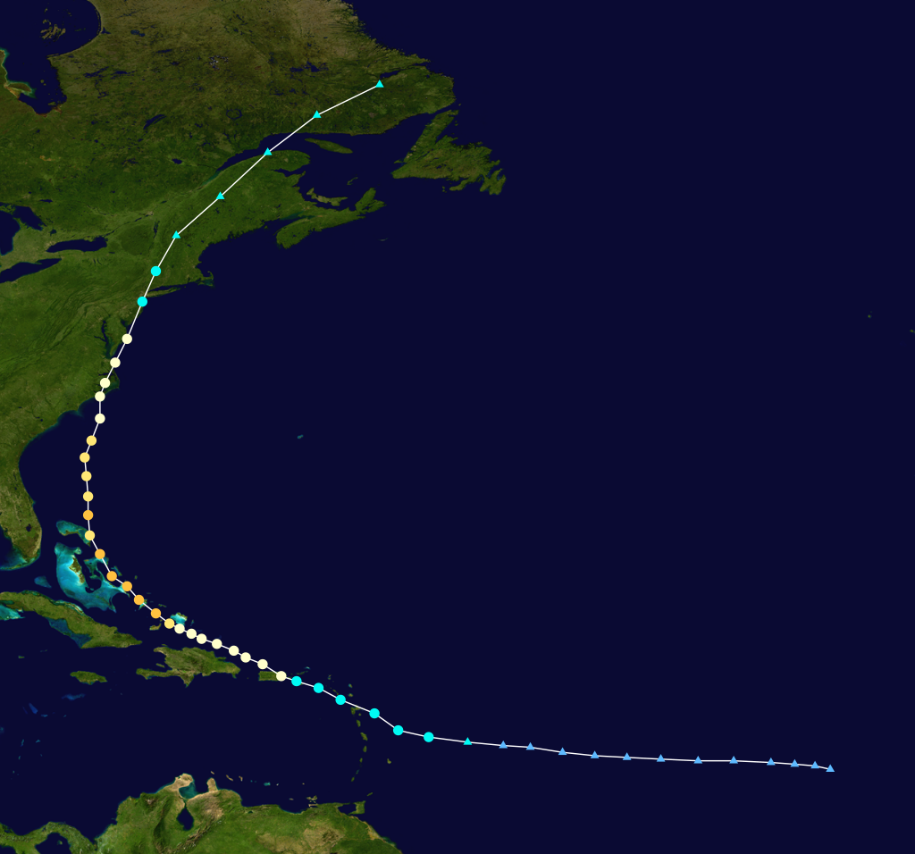
In one example of the real benefit for emergency management officials, US Coast Guard Admirals used the real time results results in their decision to evacuate their command center near Norfolk, VA, relocating to their secondary command center in Missouri. Subsequently, the predicted flooding did occur, rendering the abandoned USCG command center useless. In summary, the USCG was able to maintain uninterrupted command and control over the course of Hurricane Irene from their alternate command center, and have lauded the ASGS system for its real time contribution to this successful operational decision.

The discretization of the North Carolina domain (the mesh) that was used for both ADCIRC and SWAN is shown below in figure 4. The mesh contained 295328 nodes and 575512 with a minimum element size of 13m.

.The domain discretization for the North Carolina coast consists of 295328 nodes and 575512 elements with approximately 90% of the nodes lying near, on, or inland of the North Carolina coastline. [caption="Figure 9. "] image::http://www.seahorsecoastal.com/figures/ncv6b_mesh.png[align="center",width=400]

The land cover data that were used to derive directional wind roughness lengths, canopy coefficients, and Manning's n friction values are shown in Figure 10. The system set 127 points throughout the domain for sampling the model output for comparison with tide gauges and water levels in river flood plains and other locations. It also specified 99 locations for point sampling of model meteorological data for comparison with physical meteorological data collected at land based and buoy-based meteorological data collected by various state and federal agencies and universities.

.The land cover data for North Carolina were used to construct a complete map of directional wind reduction factors, canopy coefficients, and Manning's n friction parameters at every node in the mesh. [caption="Figure 10. "] image::http://www.seahorsecoastal.com/figures/nc_landcover.png[align="center",width=400]

The bathymetry contours are shown below in Figure 11.

.The bathymetry of the ADCIRC+SWAN mesh shows the wide range of elevations that are present; the inland extent of the mesh provide detailed coastal inundation coverage as well as river flood plain coverage. [caption="Figure 11. "] image::http://www.seahorsecoastal.com/figures/ncv6b_bathy.png[align="center",width=400]

As the storm that would eventually become Irene was forming, the ASGS had already been running for months at RENCI on the blueridge machine, a 1408 core Dell High Performance Computing cluster, producing daily forecasts using NCEP NAM meteorology, river flow data from NSSL, and tidal forcing.

When Irene formed and the decision was made to start running vortex-forced tropical cyclone forecasts, a new instance of the ASGS was started up from the most recent hotstart file from the existing NAM results.

The new instance was configured to run on 384 processors, rather than the 180 that were used in the NAM runs. Both ASGS instances then ran side by side for several days, sending their output to the CERA web application for post processing and presentation, until the NAM instance of the ASGS was shut down to conserve processor time.

On 384 processors, the ASGS was able to perform all file manipulations for the nowcast and forecast cycle for the consensus track, submit the jobs, and generate results for a 5 day forecast in 1 hour 15 minutes from the time the NHC forecast/advisory was issued.

As hurricane Irene approached the North Carolina coast, the team member that operates of the ASGS system lost electric power and could therefore no longer oversee the operation of the ASGS during this critical period. However, since the ASGS itself was actually executing at the RENCI facility, which is located in Durham, North Carolina and that facility never lost power, the ASGS was able to continue operating autonomously without interruption and without interaction or oversight for the remainder of the storm.

The results produced by the ASGS were converted in-situ to Google Earth (kmz) graphics and posted to the OpenDAP server at RENCI for use by the Newport NWS forecast office. The raw data in NetCDF format were also posted to the OpenDAP server and then a notification email was sent to the CERA web application.

The web application picked up the latest raw data, generated the image tiles for the animations and maximum values visualizations at all levels of detail, and sent email notification to selected official end users at NOAA and the USCG to notify them that new results were available for interaction over the web. The CERA website itself was not password protected, but end users were instructed not to publicize the availability of the site. The CERA web processing required another 1 hour and 15 minutes to generate image tiles for a particular advisory, for a total turn around time of 2 hours and 30 minutes.

A few comparisons with measured data are provided here; these particular plots and comparisons were developed by Kendra Dresback.

.The track of hurricane Irene was well forecast, with minor variations from advisory to advisory. The numbers on this plot indicate the locations where measured data were collected and compared with point samples of model output. [caption="Figure 12. "] image::http://www.seahorsecoastal.com/figures/irene_track_comparisons.png[align="center",width=400]

.Comparison of the forecast results from several advisories to the measured data at Oregon Inlet, NC. [caption="Figure 13. "] image::http://www.seahorsecoastal.com/figures/irene_oregoninlet.png[align="center",width=400]

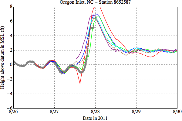
.Comparison of the forecast results from several advisories to the measured data at Beaufort, NC. [caption="Figure 14. "] image::http://www.seahorsecoastal.com/figures/irene_beaufort.png[align="center",width=400]

.Comparison of forecast results from several advisories to the measured data, illustrating the convergence of storm surge guidance so to the measured values as the uncertainty in the meteorological forecast is reduced. [caption="Figure 15. "] image::http://www.seahorsecoastal.com/figures/irene_advisory_comparisons_scatter_45deg.png[align="center",width=400]