[논문링크] (https://ieeexplore.ieee.org/stamp/stamp.jsp?tp=&arnumber=8681104)

The first to investigate a deep learning approach for dynamic survival analysis with competing risks on longitudinal data

• Dynamic-DeepHit는 longitudinal data로부터 time-to-event distribution을 학습하여, dynamic한 survival prediction을 할 수 있다.
  (dynamic이란 새로운 measurement가 들어왔을 때 prediction이 가능하다는 말인듯)
• 각 covariate(feature)가 각 event(risk)에 얼마나 영향을 미치는지 interpretation도 가능하다.
• longitudinal measurements의 temporal importance도 알 수 있다.
  

• 어떤 사건의 발생 확률을 시간이란 변수와 함께 생각하는 통계 분석 및 예측 기법
  -> 데이터로부터 생존함수,위험함수를 추정하고 해석하는 것
  -> 관심있는 event의 발생시간과 covariate(feature)와의 관계를 알려줄 수 있음.
• ex) 신규 가입 고객이 서비스를 언제(time)까지 이용할지(생존),언제 고객이 이탈할지(event = risk) ,어떤 활동(covariate = feature)이 고객 유지(생존)에 영향을 미치는지 분석,
  • survival function(생존함수) : 시간 t 이후에 생존할 확률
  • hazard function(위험함수) : 특정시간 t에 event가 발생할 확률 -> 예를 들어 event가 고객의 이탈일 때 위험함수 모양을 보고 고객에게 이벤트나 혜택을 제공할 타이밍을 결정할 수 있음.
  • Survival analysis(생존분석)with competing risks(event) :
    • event가 여러개인데, 동시에 일어나지는 못함. 예를 들어 사망원인.-> categorical한 컬럼은 모두 이벤트가 될 수 있을 듯
  • CIF(누적위험함수) : t 시점 전까지 고객이 이탈할 확률을 모두 더한 것.
    

• 매년 데이터가 측정 되더라도, 보통 last available measurement를 기반으로 분석됨.
  -> it is essential to incorporate longitudinal measurements rather than discarding valuable information recorded over time, this allows us to make better risk assessments on the clinical events.

• still maintain a propotional hazard assumption -> 시간과 관계없이 위험함수가 일정하다는 가정

• not fully dynamic; survival predictions are only available at the predefined landmarking times, not at times at which new measurements are obtained.
• it makes assumptions about the underlying stochastic process for the survival model, which may not be true in practice -> limiting the model in terms of learning the relationships between the covariates and events of interest.
• only incorporates a subset of the longitudinal history up to the landmarking time, which may result in information loss when making predictions

• provide only static survival analysis: use only current information to perform the survival predictions and most of theworks focus on a single risk rather than multiple risks.

DynamicDeepHit learns, on the basis of the available longitudinal measurements, a data-driven distribution of first hitting times.

• observed covariates

  • static (time-invariant) and time-varying covariates that are recorded for a period of time

• time-to-event(s) : 불연속적이고, irregularg하고 t_max 즉 limit이 있는 데이터
• a label indicating the type of event (e.g., death or adverse clinical event) including right-censoring.

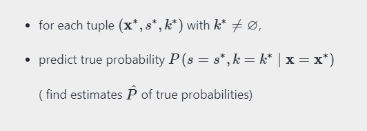
• probability that a particular event k∗ ∈ K occurs on or before time τ ∗ (conditioned on the history of longitudinal measurements X ∗)
• longitudinal measurements have been recorded up to t∗_J
• x 특성을 가진 샘플이, t시점 내에 이벤트 k가 발생할 확률을 구하는 것
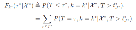
• CIF true값 몰라서 추정값 쓸거임.

• learns, on the basis of the available longitudinal measurements, a data-driven distribution of first hitting times of competing events.
• learns the complex relationships between trajectories and survival probabilities

• • Competing risks are not independent and must be treated jointly

• handles the history of longitudinal measurements and predicts the next measurements of time-varying covariates
• encodes the information in longitudinal measurements into a fixed-length vector (context vector) using RNN
• We employ a temporal attention mechanism [18] in the hidden states of the RNN structure when constructing the context vector
  • access the necessary information, which has progressed along with the trajectory of the past longitudinal measurements, by paying attention to relevant hidden states across different time stamps

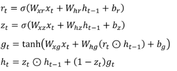
• GRU
  • 
• For each time stamp j = 1,...J − 1, the RNN structure takes a tuple of $(x_j , m_j , δ_j )$ as an input and outputs $(y_j , h_j )$ , where y_j is the estimate of time-varying covariates after time $δ_j$ has elapsed, i.e., $x_j+1$ and $h_j$ is the hiddenstate at time stamp j

• to unravel temporal importance of the history of measurements in making risk predictions

• Input : shared Sub-network를 통과하고 나온 context vector와 the last measurements
• 대상이 되는 Event의 개수만큼 Cause-Specific Sub-network를 구성(기존의 생존분석 방법들과는 달리 여러 이벤트에 대해서 분석할 수 있다는 점이 DeepHit의 강점이었음)
• 각 Event별 Cause-Specific Sub-network를 통과
• estimate the joint distribution of the first hitting time and competing events that is further used for risk predictions.

(= probability of the first hitting time of a specific cause k)

• Event 별 Output Layer 벡터들을 모두 이어붙이고, Softmax 함수를 통과
• 이걸로 CIF 추정값 구해

• 이벤트 발생 시간에 대한 Loss 함수
• the negative log-likelihood of the joint distribution of the first hitting time and events, which is necessary to capture the first hitting time in the right-censored data
  • (not censored; i번째 샘플이 이벤트가 발생한 경우): captures both the “event” & “time” at which the event occurs -> 이벤트가 발생하는 시간을 잘 맞출수록 Loss 함수가 감소
  • (censored ; i번째 샘플이 이벤트가 발생하지 않은 경우): captures “time” censored -> 이것은 Censoring 데이터(이벤트 발생 여부를 모르는 데이터)에 대하여, 관측 시점 이전까지 아무 이벤트도 발생하면 안되게 하는 Loss 함수

• 이벤트가 발생한 시점이 다른 두 샘플로부터 이벤트 발생 순서를 맞히는 Loss 함수
• i번 째 샘플이 j번 째 샘플보다 이벤트 k가 먼저 발생했을 때에 A는 1을 반환하고, 두 샘플의 CIF 추정치의 차이가 클수록 L2가 작아짐. 즉, 모든 샘플 쌍들의 순서를 맞히는데, CIF 추정치의 차이가 최대한 커지도록 Loss 함수가 설계
• concentrate on discriminating estimated individual risks for each cause
• estimated CIFs calculated at different times
• to fine-tune network to each “cause-specific estimated CIF”
• penalizes incorrect ordering of pairs
• adapts the idea of concordance ( = patient who dies at s should have higher risk at time s , than a patient who survived longer than s )
  • coefficients αk : chosen to trade off ranking losses of the k-th competing event
    • assume here that the coefficients αk are all equal (i.e. αk=α )
  • η(x,y) : convex loss function
    • use the loss function η(x,y)=exp(−(x−y)σ. ).

• incorporates the prediction error on trajectories of timevarying covariates to capture the hidden representations of the longitudinal history and to regularize the network.

• UK Cystic Fibrosis Registry
• 5,883 patients
• between 연간 2009-2015.