Week 08 (W53 Jan18) Global Climate Dataset

1- Summary

This week what we tried to reduce the dimensionality of our variables and determine the most important variables contributing in Tavg rise in the respective countries around the world. As we don't know a priori which of the methods yields the most optimal result with regards to accuracy and performance, we execute all of the necessary steps for both approaches (PCA/PCR and PLSR). As a measure of how well the output vector is approximated we used the Pearson Correlation Coefficient (or PCC). The PCC is defined as: , where cov is the covariance and σ the standard deviation. The value of the PCC can range from -1 to +1, with the plus sign denoting that Y grows linearly with X. In case of a negative PCC the Y would fall with increasing X. Either way, if the absolute value is large (i.e. close to |1|) it means that the correlation is high and therefore the scattering low. In our case we calculate the PCC between the fitted and the observed response (so X="fitted Y" and Y="observed Y" in the above equation). For this reason we want to find out at which point the PCC reaches its maximum, while discarding a variable in every iteration. So in every iteration, we discard the variable with the smallest weight and calculate the PCC. The outcome can be plotted and analyzed for a maximum. The corresponding X-value of the maximum gives us the amount of variables we can drop in order to preserve the maximum PCC.

Finally, we attempted to create a linear regression model for the emissions over the years based on our environmental data from 1960 to 2016. We used spline interpolation of order 2 for filling the missing values. Trained data from 1960 to 2006 and tried to predict 2007-2016. However, our results show big errors and we have to rethink our approach and examine different curve fitting or manipulate the training/test data size.

2 - Dataset Stats

Global Climate Data (GCD) : Main Dataset

• Number of files: 100.791
• Format: .dly files (Complete Works Wordprocessing Template)
• Size: 26.5 GB
• Features: 46
• Source Date: 1763 - 2015

World Bank (WB) : Complementary Dataset

• Number of files: 1
• Format: .csv
• Size: ~15 MB
• Features: 82
• Source Date: 1960 - 2015

3 - Data Analysis

the above plot suggests that PLSR with 4 components explains most of the variance in the observed y.The fitted response values for the 4 component model. As can be seen here PLSR and PCR are showing equal estimation accuracy with the four components. Although, it's often said that PLSR is more efficient in predicting with less number of components but for our case it is not seen till now or it is not that much visible.
![] (https://github.com/magiob/DataMining/blob/master/NewFolder.1/percentage%20variance.jpg) But, here on this you can see the actual difference. PCR being above suggests why it works poorly with less number of components as it ignore the information in the data that is important in fitting the observed y.

It's often useful to choose the number of components to minimize the expected error when predicting the response from future observations on the predictor variables. Simply using a large number of components will do a good job in fitting the current observed data, but is a strategy that leads to overfitting. Fitting the current data too well results in a model that does not generalize well to other data, and gives an overly-optimistic estimate of the expected error. Cross-validation is a more statistically sound method for choosing the number of components in either PLSR or PCR. It avoids overfitting data by not reusing the same data to both fit a model and to estimate prediction error. Thus, the estimate of prediction error is not optimistically biased downwards. But here it is not possible to reduce dimension to less than five atleast.

K mean cluster showing countries segregated in accordance to Tavg rise.It shows the clusterisation of the countries based on the centroid calculated for the Tavg rise of all countries around the world.Yellow color shows countries with less Tavg rise ,Violet color shows countries with greater Tavg rise than yellow one and blue one shows countries with midium Tavg rise and the red one finally shows the countries with the highest Tavg rise.

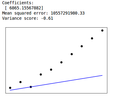
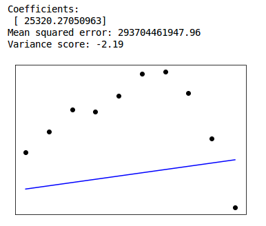
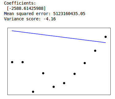
4 - Failure of linear regression model for emissions

This week we tried to create a linear regression model for the emissions of the biggest contributors (USA, China, India, Russia, Brazil, Germany) over the years. However linear regression gave very big errors. Due to limited yearly data (1960 to 2016) we have 56 values for each emission type. We also had to use linear spline of order 2 interpolation to fill in the missing values. What we did is divide our data into two parts. First train data from 1960 to 2006 and secondly predict 2007 to 2016. We would have to try exponential or logarithmic curve fitting for our cases. Problem is it seems like the trend during the latter years is turning over in compare to previous ones. Also the fact that we have little data to train and test, play a major role in the increased errors. The results are shown below.

Brazil

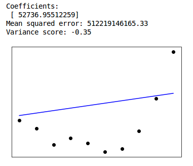
USA

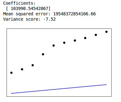
China

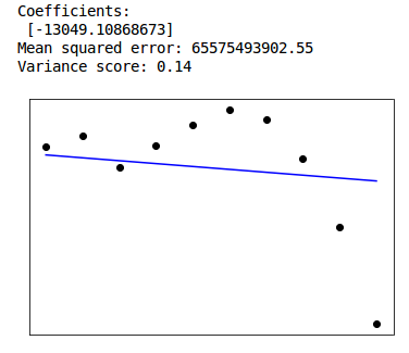
Russia

India

Germany

5 - Next Week Goals

• Keep working with the prediction model, try alternatives to linear regressions
• Train for more years, predict one year

6 - Presentation Link

https://docs.google.com/presentation/d/1M13c3j9F6-leLRTgoSktYTPeHUNqAyJDxIVoPlv7ius/edit#slide=id.p

References

1. Menne, M.J., I. Durre, R.S. Vose, B.E. Gleason, and T.G. Houston, 2012: An overview of the Global Historical Climatology Network-Daily Database. Journal of Atmospheric and Oceanic Technology, 29, 897-910, doi:10.1175/JTECH-D-11-00103.1.
2. Menne, M.J., I. Durre, B. Korzeniewski, S. McNeal, K. Thomas, X. Yin, S. Anthony, R. Ray, R.S. Vose, B.E.Gleason, and T.G. Houston, 2012: Global Historical Climatology Network - Daily (GHCN-Daily), Version 3. [indicate subset used following decimal, e.g. Version 3.12]. NOAA National Climatic Data Center. http://doi.org/10.7289/V5D21VHZ
3. WB Dataset - http://data.worldbank.org
4. Correlation Analysis - http://sphweb.bumc.bu.edu/otlt/MPH-Modules/BS/BS704_Multivariable/BS704_Multivariable5.html
5. Climate change impacts on Austrian ski areas, Robert Steiger & Bruno Abegg (Link)
6. HFCs? Curbing Them Is Key to Climate-Change Strategy (Op-Ed), Hallie Kennan, Energy Innovation: Policy and Technology (Link)
7. How do we know more CO2 is causing warming? (Link)
8. Does CO2 always correlate with temperature (and if not, why not?)
9. Earth itself is telling us there’s nothing to worry about in doubled, or even quadrupled, atmospheric CO2
10. China Exports Pollution to U.S., Study Finds