Week 05 (W50 Dec14) Crimes in the UK - Rostlab/DM_CS_WS_2016-17 GitHub Wiki
Week 04+05 (W50 Dec14) Crimes in the UK
Note: For unknown abbreviations and terms, please consider the glossary. If anything is missing, just create an issue or write us an email and we will add it. A list of our data attributes can be found here.
Content
- Cleanings and Data Preparation
- Demographic Data
- [Follow up: Random forest for predicting crime outcome] (#follow-up-random-forest-for-predicting-crime-outcome)
- Data analysis from a new angle
- [MonetDB and Rapidminer] (#monetdb-and-rapidminer)
- [Next steps] (#next-steps)
Cleanings and Data Preparation
In order to clean up the mess in our data, that we have made in the last few weeks, we reinstalled and reinitiated our database. Thereby, we considered several small findings according problems in the dataset and performed some cleanings.
In outcomes, there are 2,547,000 “crime_id”s that exist more than one time. In streets, there are 145,000 such cases. The tuples with the same “crime_id” are very similar, so that we assume that they concern the same crime and that they accrued because of updates. Therefore, we removed the older tuples. In total, we removed 656,000 tuples in streets and 3,405,000 tuples in outcomes.
We also removed all tuples before September 2011 because in September 2011, a lot of new types of crimes were introduced. We deleted 5,069,000 tuples in streets.
We dropped the column “reported_by” in outcomes, because it has always the same value like “falls_within”. Moreover, we dropped “context”, because the values are not very meaningful and is null in 99.64% of the cases.
Streets and outcomes have beside of the coordinates-columns also a column named “location”, that contains a small description of a place. In some cases, the same place have different location values, because some values are different spelled (e.g. “On or near Moretons Lane” and “On or near Moreton'S Lane”). We corrected the differences.
In the data sets from September 2013, “lsoa_code” is sometimes missing although a corresponding lsoa does exist and is given in other tuples with the same coordinates. We corrected it.
Crime Types Changed

The time series above show the evolution of the number of crimes for each crime type. As it can be seen, the crime type “Public disorder and weapons” was splitted into “Possession of weapons” and “Public order” in April 2013. We want to have data for the whole period of time. Therefore we had to merge some of the columns. We decided to merge the splitted columns again to “Public disorder and weapons”. Furthermore, the crime type “Violent crime” was removed by the police.uk since May 2013. Instead, “Violence and sexual offences” was introduced. Again, we decided to merge them and name them as “Violence and sexual offences”.
Demographic Data
This week we added "Local Authority" as a new granularity to our existing 4 levels (Lat/Lng, LSOA, MSOA, Postcode area, and region). We included the demographic data about the local authorities in the UK provided by the Office of National Statistics in the UK in their 2011 Census (link). The demographic data presents key results in the topics of population, ethnicity, health, and housing & accommodation. The data introduces the following information about each local authority (LA):
- General information:
- Population
- Number of males/females
- Number of household, communal, schoolchildren
- Number of hectares and density
- Age distribution:
- Broken down to the following ranges [0-4][5-7][8-9][10-14][15][16-17][18-19]...
- Age mean and median
- Living arrangement:
- Number of living couples, singles, married, separated, divorced, widowed
- Ethnicity group:
- Number of English, Irish, Gypsies, mixed, Pakistani, Bangladeshi, Chinese, African, Caribbean, Arab, others
- Household:
- Age distribution: Yong, old, all
- Number of cars in households: None, 1,2,3, or more
- Religion:
- Number of Christians, Buddhists, Hindu, Jewish, Muslim, Slikh, other
- Qualifications and students:
- Number of people with the different qualifications broken down into 4 levels
- Number of school children broken down into age ranges
- Number of employed, unemployed, and inactive students
- Occupation:
- Number of managers, professionals, associates, administratives, skilled, caring, sales
- Length of residence in UK: (values from 2011)
- Number of people born in the UK
- Residents less than 2 years, less than 5 years, less than 11 years, and more than 10 years
Follow up: Random forest for predicting crime outcome
In our previous Wiki we described our first approach for predicting crimes outcome. we narrowed our experiment to the city of London (~21,500 samples), which we splitted into training and test datasets. We created a random forest with the help of the Scikit-learn Machine Learning library. We chose the following features as an input set: Crime type, number of POIS, and the three most effective outcome types of stop and searches incidents. As a result 10 decision trees were generated with i) cross validation accuracy on the training data set: 59%, ii) accuracy on the test dataset: 95.9%, and iii) weighted F1-score for the prediction model: 0.76478.
As planned, this week we analyzed the random forest and enriched it with the new data. Here are the respective findings:
-
Incorrect accuracy on the test dataset for the city of London: We discovered a bug in our python code that resulted this high, yet false, prediction accuracy on the test dataset. Instead of comparing the predictions and true values of the test data, we only compared the first binary vector of the encoded crime_type (that was transformed to 15 binary columns using the OneHotEncoder). The correct test data accuracy of the initial random forest is 55.9% and not 95%
-
Enrichment of the data:
- Input - categorial features: Crime type, postcode, local authority name
- Input - 174 numerical features:
- Number of stop and searches within 500m broken down by outcome type, ethnicity, person and vehicle searches.
- Number of Points within 500m of Interest broken by the respective types.
- Number of crimes in the respective postcode area broken by crime types
- Demographic information in the respective local authority as mentioned in section 1
- Prediction goal: crime outcome
- Sample size: first we executed the script on the whole dataset ( ~ 35 Million samples). However, after receiving a memory error on the server, we drawn a sample of 5 Million entries
- New results:
- Accuracy of training data: 54.8%
- Accuracy of test data: 55.2%
- Weighted F1-score 0.544804294657
- Confusion matrix: The following confusion matrix summarizes the performance of the random forest on the test data. Each row presents the number of correct and incorrect predictions broken down by each crime type. It shows in which way our random forest is confused when making predictions. The information in the matrix corresponds to the low prediction accuracy.

- Image first tree: The following image shows the first 3 nodes of the first generated tree in the random forest. Interesting to see here is that the first splitting node changed (compared to last week) after including the new demographic data

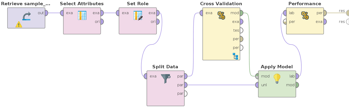
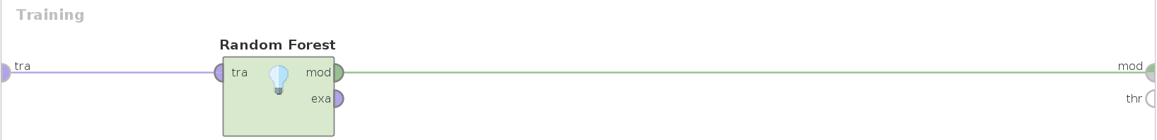
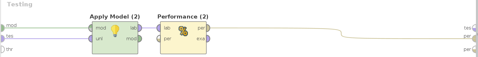
- Our current interpretation/conclusion: We suspected that one can’t properly predict a crime outcome based on the data we have, which doesn’t include essential information about the crime like: Perpetrator’s and victim’s age, ethnicity, criminal and psychological history, witness statements, etc.. . This first prediction experiment confirmed that there are no correlation between the input features and the crime outcome. However, it was interesting to observe that the implemented random forest was not able to reach 65% accuracy (since 65% of the outcome type is “Investigation complete”), but Rapidminer was able to reach this expected number.
Data analysis from a new angle
Since that predicting crime outcome is not feasible with the current data, at least in the current form, the newly added demographic data about local authorities in section 1 gave us the opportunity to look at our data from a different angle - namely location based.
This week we computed the Correlation matrix with the following rows that represent data about the different granularity levels:
- 500 m around crime:
- Average number of stop and searches broken down to outcome types, age ranges
- Average number of POI broken down into the different categories
- Postcode areas:
- Average number of crimes in postcode areas broken down to crime types
- Local authority:
- Average of demographic information introduced in section 1
The rows of the correlation matrix consist of mainly the absolute and relative (per 10,000) number of each crime type. To compute the table we used RapidMiner. Our correlation matrix can be seen here. For example the table shows a high correlation (~0.8) between the average number of Points of Interest and the number of crimes per 10,000 persons. It’s surely not a surprise. Furthermore, the table also shows a very strong correlation (~0.9) between the number of males in local authorities and the absolute number of crimes. However, by considering the number of crimes per person and not the absolute number, it shows a non-significant correlation of 0.15
Furthermore, we have created 16 maps, each of which visualizes the distribution of a specific crime type per 10,000 person in every local authority in the UK. The following two maps for example show the distribution of the crime types “anti social behavior” and “Vehicle Crime”
-
Anti Social behaviour per 10,000 person:

-
Vehicle Crime per 10,000 person:

Based on the correlation matrix and the crime type maps we still can’t conduct any direct statements. Yet we believe that they shall serve the new, location-based, prediction goals.
MonetDB and Rapidminer
MonetDB
Since this week, our dataset has a volume of about 35 GB (as CSV file) in a single table - that is quite a challenge for our own machines with 8 to 16 GB RAM. Although our scripts to generate map illustrations or to do intelligent things (e.g., decision trees) are written in Python, our main tool to transform and analyze the data is a relational database.
Started with MySQL in the first week, we recognized soon, that it did not fulfill our requirements: we could not even join two of our initial tables. Therefore, we have used PostgreSQL in the 2. and 3. week. With it, we could perform some spatial joins and do all joins and group by/aggregations we wanted to; but it was slow. We needed about a half hour to import or export our data set, often also up to a half hour for simple group bys, and 6-8 hours to fill a new table with joined data. That made it very hard for us to define our analysis-questions and to answer them in the same meeting - even if the meetings took a complete day.
MonetDB - our third database management system. But now, we think that we have found the solution. As we have learned in our database lectures, we knew the advantages of column stores for analytical queries. Therefore, we decided to try MonetDB, that uses such a column store and techniques like "vector at a time" instead of "tuple at a time" and seems to be optimized for data mining problems.
It was a pleasant surprise! Although, our machines have not more than 16 GB main memory, MonetDB showed a much better performance than PostgreSQL. We were able to export and import our dataset in about 4 minutes, and the most aggregation queries only took under a minute. It has not the broad range of features of a MySQL or PostgreSQL database or an own GUI, but all functions we need. Therefore, we hope that it would be able to have it on the server machine and also recommend the other groups to give MonetDB a try.
RapidMiner
As we have mentioned above, we have used RapidMiner to computed the correlation matrix. Furthermore, we tried to use it for doing some computations. Unfortunately, we got a memory error for the most algorithm, even for a small sample of our data. Therefore, we are going to try to utilize RapidMiner on the server.
Next steps
- Analysis and predictions from a new angle - namely location based:
As the results of the random tree showed us, the available input features are not sufficient enough to predict crime outcome types. So far we had crime types in the center of our project. Now, with the help of the aggregated crime and demographic data about the different location granularities, we will shift our focus to location based analysis and predictions.
- Data transformation: In order to fulfill the location-based approach, we will work on the possible feature transformation and data preparation.^