Week 04 05 (W50 Dec14) Global Climate Dataset

1 - Summary

This week we focused on analyzing data for Austria. A major reason for this choice is that Austria is a country affected greatly by climate change, due to its big dependence on snowfall for winter tourism. There are many reports about the shrinking of winter season and the financial damage on the country (https://summitcountyvoice.com/2014/09/20/is-austria-a-climate-change-hotspot/). Another reason is that Austria is a small country, whose data we can manipulate more effectively, in comparison to India which has an abundance of data including a lot of bad data. We collected all data existing (features: TMIN, TMAX, TAVG, PRCP, SNOW, SNWD) for Austria from the GCD dataset. These include the cities of Kremsmuenster, Wien, Salzburg, Innsbruck, Sonnblick, Graz, St. Poleten, Feuerkogel, Villacheralpe, Klagenfurt. We further did analysis of the data, converted them to yearly and merged them into a single dataframe. In addition to this, we employed the WB dataset and extracted ~80 environmental features, which we merged also into a common dataframe with GCD data. Finally we did correlation analysis for multiple features of both datasets.

2 - Dataset Stats

Global Climate Data (GCD) : Main Dataset

• Number of files: 100.791
• Format: .dly files (Complete Works Wordprocessing Template)
• Size: 26.5 GB
• Features: 46
• Source Date: 1763 - 2015

World Bank (WB) : Complementary Dataset

• Number of files: 1
• Format: .csv
• Size: ~15 MB
• Features: 82
• Source Date: 1960 - 2015

3 - Goals Achieved This Week

• Extraction and merging of all Austrian data
• Merging with WB dataset
• Analysis of data
• Correlation analysis

4 - Analysis of Data

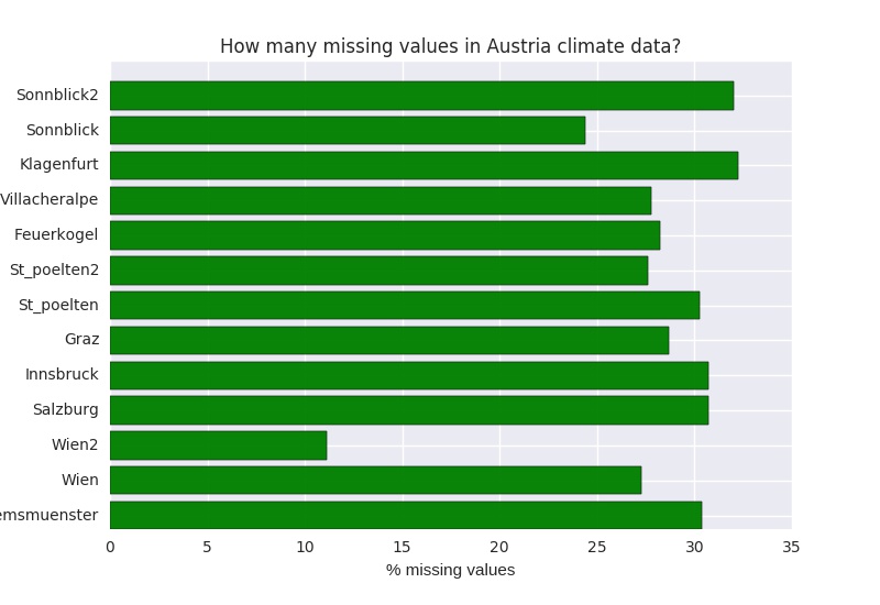
First we estimated the percentage of missing values for each city of Austria available. We observe that each city has on average around 27% missing values.

More specifically, we captured the matrix of missing values for the city of Wien. We see that most of the missing values are in the TAVG and SNOW features.

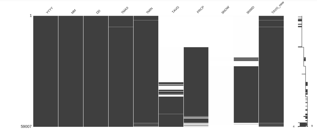Missing values matrix for Wien dataset

However, we also have a second dataset concerning Wien. The missing values matrix of the latter is the following. Here missing values exist only in TAVG feauture, while SNOW is complete.

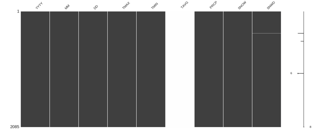Missing values matrix for a second Wien dataset

Therefore, it is wise to merge these two datasets since they refer to the same city. At the same time we observe that TAVG feature which is the average temperature has mostly missing values. Thus, we decided to make use of the TMAX and TMIN, which are the maximum and minimum temperatures respectively to compute a new average temperature. We did this for all the cities included in the data.

We estimated the standard deviation per year for the features of the cities examined. Following we present the table with the standard deviation values for each feature year-wise for the city of Wien for the years 1986, 1992, 1998, 2004, 2010, 2016 (starting from bottom to top on the table)

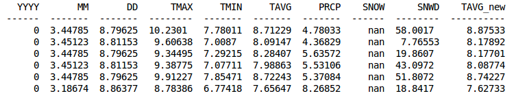Standard deviation for Wien dataset

Following as presented during previous week, we are following the option of interpolation with spline of order 2 to fill in the missing values in our data. We decided then to visualize the feature of TAVG_new (that is the average of TMIN and TMAX) to observe the trend. We present the graph for the city of Wien.

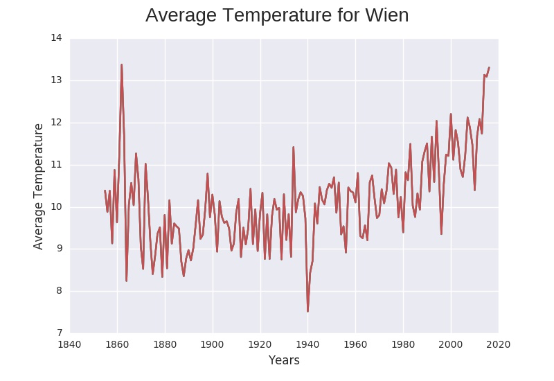
Average temperature for Wien dataset

We can see that from 1960 there is a steady rise in the average temperature. This is threat to the snow-dependent winter tourism industry of Austria. The snow melts faster and the number of ski days decrease (snow depth ≥ 30 cm). As a result snowmaking is required to balance the negative impacts. However this is still not enough as cannons cannot produce enough amount of snow for a warming higher of 2 degrees. A 2 degrees warming warming would halve the number of naturally snow reliable ski areas, and with a 4 degrees warming, expected for the end of 21st century, only a very small proportion of ski areas would remain [5].

Following we merged the common datasets for the same cities. These were Wien, Sonnblick and St. Poelten. We had to set a common index of dates YYYY.MM.DD (Years.Months.Days) and the concatenate them column-wise and at the same time estimating the mean value for each feature. In case of nan we keep the existing value of one of the datasets. Further we converted all cities daily data to yearly and concatenated them into a single dataframe. Then we extracted data related to Austria from the WB dataset and concatenated them into the same dataframe. Eventually we have a 162x150 matrix with all features per year with 69% total missing values.

Finally, we estimated the % of change in variables from 1960 to 2016. We filtered them for a degree of change greater than 30%. We observe that HFC gas emissions, CO2 emissions, and other greenhouse gas emissions have gone through a huge increase in that specific time frame. These emissions are directly related to the climate change and could be a possible cause. Particularly for HFC gas there are various reports about its dangers. These gases may make up a small percentage of the emissions society generates, but they pack a devastating punch when released. The threat level for each of these gases varies based on several factors, most notably their lifetime in the atmosphere and their potential to influence global warming . Reducing the emissions of those gases in addition to those from carbon dioxide is critical to achieving a stable climate [6]. In addition to this, the effect of adding man-made CO2 is predicted in the theory of greenhouse gases. This theory was first proposed by Swedish scientist Svante Arrhenius in 1896, based on earlier work by Fourier and Tyndall. Many scientist have refined the theory in the last century. Nearly all have reached the same conclusion: if we increase the amount of greenhouse gases in the atmosphere, the Earth will warm up [7].

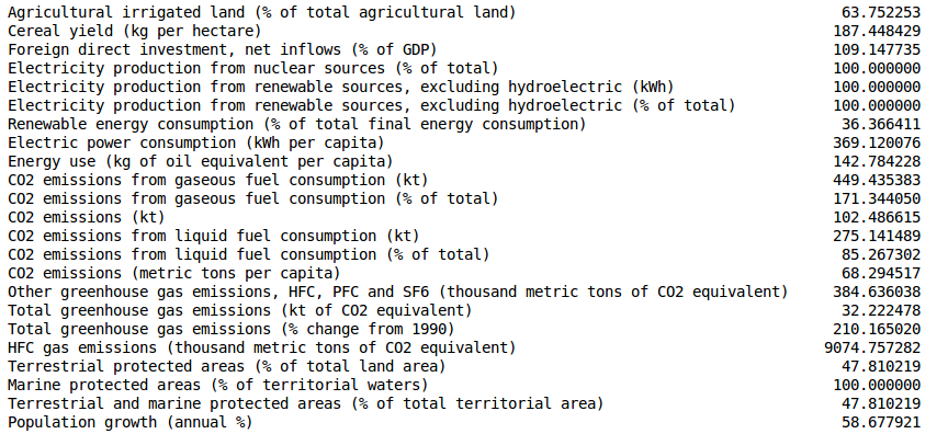% change of WB dataset features. Filtered for change > 30%

![] (https://github.com/magiob/DataMining/blob/master/NewFolder.1/Tmin.jpg) ![] (https://github.com/magiob/DataMining/blob/master/NewFolder.1/SNOW.jpg) ![] (https://github.com/magiob/DataMining/blob/master/NewFolder.1/Tmax.jpg) ![] (https://github.com/magiob/DataMining/blob/master/NewFolder.1/SNDW.jpg) City based climatic describtion of Austria

What we can see here is a variation of four climatic features along the years from 1960-2016 segregated based on cities in Austria.These graphs shows city wise variations which implicate the necessity of implementing an appropriate method for calculating the appropriate climatic values representing Austria as a whole.The interpolation used here for missing values is linear as the variation among data is on a linear format.As can be seen from the graph it is appropriate to take the mean of Tmax and snow of all cities to represent Austria as a whole because data is quite close but for SNDW and Tmin one city shows large variation in terms of values compared to other cities.

Climatic variables variation along years by taking Austria as a whole

5 - Correlation Analysis

We did correlation analysis for the data in Austria to spot consistent patterns between the variables of the two datasets in order to further filter "useless" variables and investigate others in detail. Here we present the graphs of the correlation analysis results. During the presentation more explicit explanations will be given about the positive, negative or "hard to tell" variables correlation.

6 - Next Week Goals

• Try new analysis tools for Austria data
• Improve visualization, attempt in-map visualization
• Extend features analysis

7 - Presentation Link

https://docs.google.com/presentation/d/1-EkTZLkCVLe_-u6oH7tNrgFWEK62JQB_dF19_ztodfM/edit#slide=id.g1a15825fbd_0_77

References

1. Menne, M.J., I. Durre, R.S. Vose, B.E. Gleason, and T.G. Houston, 2012: An overview of the Global Historical Climatology Network-Daily Database. Journal of Atmospheric and Oceanic Technology, 29, 897-910, doi:10.1175/JTECH-D-11-00103.1.
2. Menne, M.J., I. Durre, B. Korzeniewski, S. McNeal, K. Thomas, X. Yin, S. Anthony, R. Ray, R.S. Vose, B.E.Gleason, and T.G. Houston, 2012: Global Historical Climatology Network - Daily (GHCN-Daily), Version 3. [indicate subset used following decimal, e.g. Version 3.12]. NOAA National Climatic Data Center. http://doi.org/10.7289/V5D21VHZ
3. WB Dataset - http://data.worldbank.org
4. Correlation Analysis - http://sphweb.bumc.bu.edu/otlt/MPH-Modules/BS/BS704_Multivariable/BS704_Multivariable5.html
5. Climate change impacts on Austrian ski areas, Robert Steiger & Bruno Abegg (Link)
6. HFCs? Curbing Them Is Key to Climate-Change Strategy (Op-Ed), Hallie Kennan, Energy Innovation: Policy and Technology (Link)
7. How do we know more CO2 is causing warming? (Link)