Image_Processing - RicoJia/notes GitHub Wiki

========================================================================

Image Processing

========================================================================

Image is a function f(x,y), and you can plot their values:
- smoothing of a function = blurring of an image
- image will have a min, max, even negative nums
  - 255 is a pure incident
- image: --> x(j), | V y(i)
- MATLAB indexing starts at 1
Filter:
- average filter is always odd.
- moving average with a uniform one [1,1,1,1]*0.25, in 2d, it's called box filter
- moving average non-uniform one, with 4 in the middle, can preserve the "characteristics" [1,2,4,2,1] (middle one is the one x current val, this is also the kernel, or mask)
- in 2d, it's a "Gaussian filter"
  
  caption
- Gaussian filter will be smoother, cuz a single pixel convoluted with a gaussian filter is still a blob
  
  caption
- Note that Gaussian filter's first term (aka normalization coefficient, which affects brightness) is 1/(2pi*sigma), not 1/(sqrt(2p) * sigma)
- the word isotropic means "circularly symmetric"

size of the kernal is not "the bigger kernal", bigger here means the standard deviation of gaussian.
- the size of the kernel is the bigger the better,because it will provide smoother performance.
- the bigger the kernel, the blurrer it will be

Filters
- If a filter does cross-correlation with an impulse, you don't get "flipped version" of the impulse
  
  Impulse response is flipped!
- Convolution is when you do have filter or the image "flipped" around a pixeli (or rotate by 180 deg). you flip a filter (about the center), then move it around the image, multply and add.
- So the impulse response of a filter will be the impulse response itself
- when the filter is symmetric, cross-correlation and convolution give you the same result.
- Convolution properties:
  1. f*g = g*f
  2. f*(g*h) = (f*g)*h
  3. del(f * g) = del(f) * g, here del f = del (f)/del(x) (useful in edge detection)
- Complexity
  - a convolution: NxN filter on an MxM image, that'd be N^2M^2 multiplcations and additions
  - if you have linearly separable filter: C*R, think of the two as padded 3x3 matrices,
```
[1
 2  * [1 2 1] = 
 1]

                [1 2 1
                 2 4 2
                 1 2 1]
```
    The complexity is (C * R) * F = C * (R*F) = 2xN x M^2
- with zero-padding, dark edge will "leak in" after filtering
- Unsharp Mask: just (could be done with chemicals, because it's a blurry version of the original), then you do F - M, you will get a sharper picture
```
    [1 2 3    [1 1 1
 M=  2 3 4  -  1 1 1
     3 4 5]    1 1 1]
```
- Median filter: to remove salt-pepper noise (random spikes here and there), by finding the median of the neighbor. Because here we're assuming image as a function should be "continuous". We also call it edge-preserving
Filters as templates
- A template is a "pattern" that we're looking for. When a filter cross-correlates itself, it gets its highest value when being with a similar pattern
- The technique we use is called "normalized correlation": Normalised_CrossCorr = (1/N)*sum((x-mean(x))*(y-mean(y)))/(sqrt(var(x)*var(y));
  1. Scale all filter values so their standard deviation become 1
  2. Scale the local patch values so their standard deviation become 1 as well
  3. do the correlation across the image, and find the patch with the highest value
- template can only work for the exact same images

========================================================================

Morphology

========================================================================

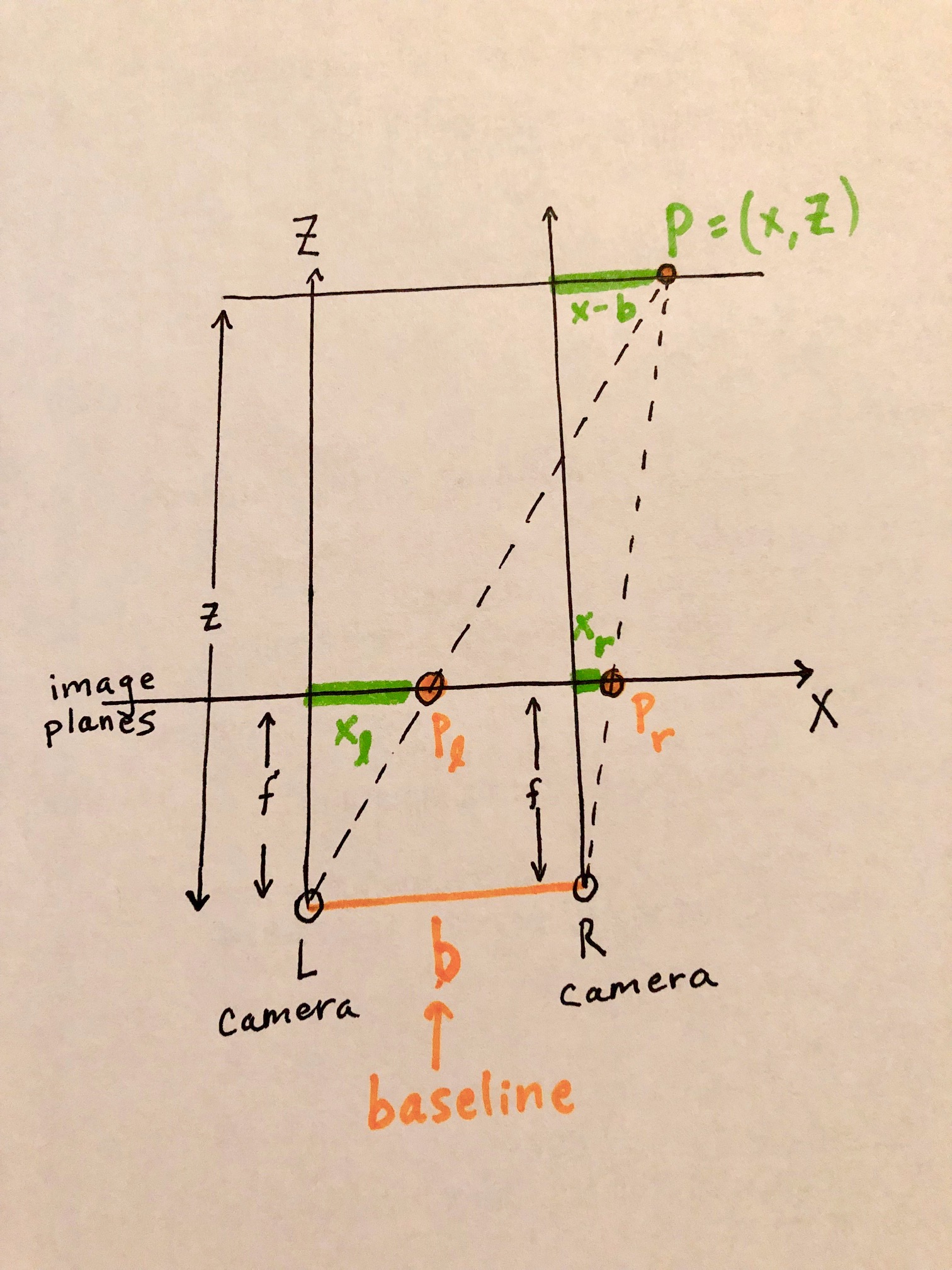
disparity: In Stereo Vision, disparity is the difference in pixel of the same point, x_l - x_r
1. Have a window (xl) to compare similarity for
2. Going along epipolar line, in a search region, slide along the window, find window (xr) has the highest similarity score
3. For pixel xl, the disparity value is |xr-xl|. That's the disparity value
4. **A good general workflow is: ** fish eye camera view -> projection (fish eye to surface projection will cause downscaling) -> ROI generation (thresholding disparity values) -> ROI mask (reproject the mast back to the fish eye view)

========================================================================

Edge Detection:

========================================================================

edge is sudden decrease/increase in pixel values, perpendicular to the image gradient
- a gradient in image is by using the difference equation: (f(x+1) - f(x)/1) = (f(x+1) - f(x))
- so you can use a small filter: x direction: [-1,1], y direction [-1,1]T (assumey is going down from top left corner)

Sobel Operator

Sobel Operator is an edge filter:

  G_x: : comes from a smoothing filter [1,2,1]/4 and [-1, 0, 1]/2 (see above for the 2)
  [ -1, 0, 1]
  [ -2, 0, 2] * 1/8
  [ -1, 0, 1]

  G_y: 
  [ 1, 2, 1]
  [ 0, 0, 0] * 1/8 (y goes up, which is the opposite of the above direction)
  [ -1, -2, -1]

  Ax = G_x * A  (A is original image, * is correlation, convolution will flip the image, but if you flip the filter first, doesn't matter)
  Ay = G_y * A  (A is original image, * is correlation)
  G = sqrt(A_x^2 + A_y^2)   (this is the gradient at each pixel, A_x, A_y are pixel values)
  theta = atan(A_x/A_y), the direction of the gradient (atan2)

the 1/8 is important, otherwise normalization will not be correct, and edges will be wrong
In real life, you just calculate G at each image, then plot it, and you can even threshold
there's Prewitt, Roberts filters that're similar
- the 1/8 is important, otherwise normalization will not be correct, and edges will be wrong
- In real life, you just calculate G at each image, then plot it, and you can even threshold
- there's Prewitt, Roberts filters that're similar

Noise reduction: in real world, noise will create lots of high gradients

More edges in noisy pictures
Therefore we need to smooth the pic first: (take x direction for example) (so this is different smoothing than sobel operator)
```
del(h * f)/del(x) = del(h)/del(x) * f
```
- smoothing function h, and h' are, which will save us from a whole differentiation cycle.
- This is because differentiation allows associativity, and associaitivity allows us to get direvative of the filter.
- How do we know where there's a peak? use second derivative. We can identify extremas
  
  Second Order Derivative
- To visualize the first order derivative of the fitlers:
  
  Visualization of First Order Derivative of Smoothing Filters
- The bigger the smoothing filter, the less noise will be incorporated
  
  Smoothing Filter

Canny Edge detection:

Developed by Jhon Canny, as his masters thesis
4 steps: Smooth, Thresholding (find the significant edges), Thinning (Replace a fat edge with a thin one.), Link separate contours
1. Smoothed - image gradient (Like Sobel)
  
  Smoothing + Image Gradient
2. Threshold
  
  Thresholding
3. Thinning, aka non-maximum suppresion. I will keep the strip that exceeds the threshold the most. (i.e, find the local maxima in the edge)
  
  Thinning
  
  Thinning Result
4. Linking: Link broken Contours together, really cool
  - Two threshold for thresholding: high one for "strong" edges, low one for "weak edges". Connect strong edges and weak edges together. Here we assume we want to keep weak edges that are linked to strong edges.
  Linking

Hough Transform

finding a line! Finding a circle
- it's actually "fitting a line", because you may have gaps, noise, etc.
- each edge point will get to vote, including the noisy ones, but the noisy ones shouldn't be consistent enough for a good feature
- Hough transform vote for lines
- A point in xy space is a line in Hough space (k-b space), then you plot those lines, and whichever bin has the most votes, will win
  
  Hough Space
  
  Voting
- but y=kx+b suffers from vertical slope. So we use parametric representation: d = xcos(theta) + y sin(theta)
  
  A point in x-y space will become a sinusoid in d-theta space
  - theta: [0,2p), d>0
- Algorithm: the bins are also called "Hough Accumulator Array".
  1. Initialize each bin to 0
  2. for a given (x0, y0), iterate thru theta, then calculate d.
  3. Find the (theta, d) with the max value
- complexity: K^2 * (k bins along each dimension.)
- E.g:
  
  A perfect line is that bright spot
  
  caption
- Cautions:
  1. you may want to take a look at probablistic Hough Transform, which samples points to find the best fit.
  2. Noise can bump you off, so you may want to smooth the edges a bit more
- Extensions:
  1. use gradient imgs (del(f)/del(x), del(f)/del(y)) instead of just one edge pic, so for each edge pixel will only vote for thetas close to the gradient orientations.
  2. you can use hough transform, instead of regression, to find circles.
  3. Give stronger edges more votes
Hough Transform for a circle!
1. assume you know r, then all you do is vote for (a, b)
2. If you don't know r, then it's a pain
3. But if you have gradient, you can check if (a,b) generates a radius that corresponds to the gradient
Pros & cons:
1. pros:
  - Some robustness to noise
  - Occlusion is fine, cuz all points are processed independently
  - can detect multiple models in a single pass
2. Cons:
  - Complexity goes exponential as number of params go up
  - Detected targets can be spurious
  - difficult to pick a good bin

Generalized Hough Transform

generalized hough transform:

You have a template, and an image, you're going to search fro the template in the image.
The template has irregular shape, so you can't express it in parametric eqns.

For simple case where shape and location don't change, Instead, you express it like this:

  1. Find centroid (Xc, Yc) in template (offline)
  2. Find edges in centroid
  3. For each edge k (a,b), Calculate its distance to Xc,Yc dk, the angle of (Xc - a, Yc - b), theta_k
  4. Build an R table, based on the orientation of its gradient, Phi_i
      Phi1 (dk, theta_k)
      phi2 (dm, theta_m), (dn, theta_n)
      ....
      Because we may have parallel edges, we may have multiple entries under a single Phi
  5. In the image, identify the blobs, and find its edges. (Online)
  6. For each blob, 
        a. For each edge point on the blob, 
            1. get its gradient direction, Phi_i
            2. look up (dm, theta_m), (dn, theta_n)... under Phi_i, 
            3. then calculate the corresponding reference point (x1, y1), (x2,y2), and increase their votes. 
        b. Once you're done with all edges, find the pixel with most votes. If the votes are more than a threshold, 
        then we think: 1. the blob matches the template 2. the pixel is the location of the contour
  7. Move on to the next blob, repeat 6.

generalized Hough Transform with random scale and orientation:
1. sample scale space: S1, S2 ...
2. For each scale, do the above

edges are old. Features (code words) will be more prevalent.

  1. Features (like Harris Corner), are small image patches. They represent a code word? Equivalent to "edge" here
  2. Offline, using a centroid, features develop an R-table for codeword and displacement(feature, centroid). 
  3. Online, identify each feature, and their blobs, following the same idea.

Hough Forest: with classifiers like random forrest, using voting for displacement, orientation with features

========================================================================

Fourier Transform

========================================================================

Aliasing happens when sampling frequency is lower than 2 times of the highest fequency in the signal, like jagged lines
- a set doeson't have to be orthogonal, just independent is fine.
- fourier transform in image analysis:
  
  Lower frequency vs high frequency
- computer vision
frequency analysis
1. ringing: after removing some high frequency
Ringing
1. Getting rid of low frequency components is like edge image
"Edge images created by high pass filter"
1. accentuate low frequncy will give u stronger edges
Stronger edges with weaker low frequency components
1. Some interesting patterns
1. horizontal line in 2D FFT:
- in 1d, [1,1,1,1,1] (frequency domain) is impulse response [0, 0, 1, 0, 0]
- in 2d,it's equivalent to summing up e(...x,y) * u(x,y) along y first, then along x (order here doesn't matter) link
- a perfect fourier transform assumes periodic signal (images wrapped around and around). So if you have a dark edge at the bottom of your image, you get sharp edge on Fourier analysis.
  - use a gaussian filter (on the whole thing?)
1. multiplication in spatial/frequency = convolution in frequency/spatial
2. What is Fourier Transform? note amplitude (A), phase (phi) are both encoded in F(w)
Fourier Transform Derivation
1. If mask and image are big, use the "Fourier Trick"
2. A gaussian in spatial space is also a gaussian in frequency domain. But, the sigmal will be inverse. So: the larger spatial sigma is (of the kernel), the narrower it is in frequency domain, so the lower frequency it allows to pass.
Gaussian kernal's sigma is inversed in frequency domain
- Effect of Gaussian
1. ringing and its counterpart (which cancels ringing)
1. box filter is a sync in frequency domain. sinc = sin(x)/x. See the ripples? they cause the jagged thing in spatial domain.
- sinc in frequency is a box in spatial as well!
- So why you don't want to just cut out the high frequencies! which will introduce ringing

More Fourier Transform

One Impulse Train (Shah Function) in space is another impulse train in frequency domain
- Derivation
- when T-> 0, then there's just one impulse in time domain, and we get a solid 1 in frequency domain
- Because of shah function, Nyquist Theorem was developed afterwards.
Aliasing
1. if you have too few samples, you can't tell if it's high frequency or low frequency
2. Your eyes' framerate are not that high, so you may see wheels turn backwards, then forwards. That's aliasing
3. AntiAliasing: Use low-pass filters. This is better than aliasing.
- low pass filtering in inputing
- During reconstruction (like in audio), use low-pass filter on the output again, cuz we know the input signals should be thrown away
1. Nyquist Theorem
Convolution and Sampling

2B must < f 5. Anti-Aliasing Filter: to get rid of high freuqency components

Anti-Aliasing Filter
- Have to use it before sampling, cuz after sampling, there's no way back!
1. Application of Anti-aliasing filter: when you downsample, to keep the edges better, apply AAF before downsample
- Downsampling: take every other row, for exampe
  
  Carving out every other row, column will lost some features
- use gaussian
  
  AAF will keep the features instead of simply carving pixels out
- Might be useful for facial recognition
1. Contrast:
- contrast is the range of [low, high]
  
  Contrast is the Range of intensity values
- human eyes are sensitive to different contrasts at different frequencies. So you can leave out the high frequency high contrast stuff
  
  Low contrast elements of High Frequency Can be left out
1. JPEG uses discrete cosine transform
  - similar to Fourier Transform, DCT gets some coefficients at each frequency, for each cosine (remember fourier transform is e^(j2piw*t))
    1. disect the image into 8x8 sections
    JPEG takes 8x8 pixels
    1. for each 8x8 sections, convolve with each block in these filters: top left is low frequency, then along the x, y axes, f goes up. the rest (i,j) represents cos(f_i*f_j).
    Visualization of the JPEG filters
    Then you get a component of each frequency. This is Discrete Cosine Transform DCT only works with real values, so it's great! But certain properties wont hold
    1. Given human perception, we require different accuracies for different frequencies' components
    - "Quantize" by rounding to the nearest value, e.g, 3 at top right, so (16/3=5)
    Quantization Table

========================================================================

Implementation

========================================================================

Huffman Coding
1. The more frequently a letter (or a symbol) appears, the less bits we should use for them. So we need to know how frequently a symbol may appear
2. However, now the problem is: if H is 0, E is 00, the HE (000) might be the same as EH. So the codewords must not create ambiguity. So they call this "non-prefix code"
3. Huffman Coding comes to rescue. It generates a binary tree, Based on how frequent each char is.
4. How to form a code for a set of symbols
Forming a Huffman Tree
1. Why?
It can't be decoded into anything else, if you decode from start to end!
1. Working Example:
  - Notice how you can't decoded this into anything else: because the tree is a "full" tree, i.e, if a node has only one child, that child must be a leaf node.
2. Some things to keep in mind:
  1. Every set of symbol needs to generate a customized code
  2. And The decoder must know the code (the Huffman table)
JPEG
1. The input is a bmp image. with full on RGB values at each pixel.
2. chroma sub-sampling: we can see brightness differences well, but not color differences. So JPEG throws away a lot of colors. The output is a Y'CbCr image.
  - Y is brightness, Cb is blue components, Cr is red components. Cb, Cr are chroma components.
  - successor of YUV (1950) for transmitting analog TV signals using less bandwidth than RGB. Also, it can have backward compatiblity with black&white TV. (using the fact that if RGB values are the same, they will be a point on the grey scale)
  - chroma means "color" in greek.
  - Y, Cb, Cr can be converted from RGB values. Where the brightness of a pixel, is determined by RGB value all together. (Similar to greyscale)
    
    caption
    
    The higher a value is in dimension, the more "brightness" it has
  - So Y will be kept the same (since eyes are more sensitive to it), and Cb, Cr resolution will be decreased to save bits.
3. DCT & quantization
  - Separate an image into 8x8 chunks, then run DCT to get frequency components
    
    You can see the reconstructed images by adding the frequency components back
  - For each 8x8 section, you get one number after you convolve it with a frequency pattern. That's called a DCT term. Quantization table is how to do the rounding. We want smaller terms for high frequency components
    
    How you get frequency components for compression
  - Human eyes can't see changes occur in close proximity (high frequency components), so there're more low-frequency components, and fewer low frequency components. Quality Factor controls how big the devisors are
  - brightness is also quanized: low brightness values have lower resolutions.
  - Quality factor is how fine the quantization resolution can be
4. Huffman coding
H264 Decoding
1. Aka AVC. There's also H.265(HEVC), RM (real player 20 yrs ago ). H264 has AAC (audio), 80% from MJPEG compression
2. Will compress on portions which don't move much. (Temporal Compression)
  - iframe (aka keyframe), is pretty much the same as MPEG frames. Requires higher bit rate, lower processing power. Also known as intra-frame
  - pframes are medium size, which illustrates difference s from the previous iframe, or pframes.
  - bframes will compare itself with the previous and the next iframe, pframe, or bframe. Smallest in filesize, but will introduce latency. **Camera Manufaturer can choose if bframes are used. **
  - QP means quantization Parameter (20-51)
3. MJPEG is simply encoding frames into jpg.
4. Spatial Compression: Compare the pixel values block by block, and find matching pixels. Say if a blob moves from position A to B, h264 should be able to find it.
- Question: how does this work?

cv2

depth - number of bits to represent a pixel
- CV_32F is 32 bit float
Practice Experience:
- convolution is just flipping the kernel, pad the image on both sides, and
  - the output size should be n = (img + 2*padding_size_one_side - kernel_size +1), so we can make the output image the same size as the input image!
- cv2.filter2D applies correlation, not the real convolution.
  - also, it doesn't work with RGBA, only RGB!

Image_Processing - RicoJia/notes GitHub Wiki

Related Topics

Image Processing

Morphology

Edge Detection:

Sobel Operator

Canny Edge detection:

Hough Transform

Fourier Transform

More Fourier Transform

Implementation

cv2

⚠️ GitHub.com Fallback ⚠️

Image_Processing - RicoJia/notes GitHub Wiki

Related Topics

Image Processing

Morphology

Edge Detection:

Sobel Operator

Canny Edge detection:

Hough Transform

Fourier Transform

More Fourier Transform

Implementation

cv2

⚠️ **GitHub.com Fallback** ⚠️

⚠️ GitHub.com Fallback ⚠️