IMD Measurements - QuantAsylum/QA40x GitHub Wiki

IMD measurements are a means for teasing out non-linearities in amplifiers, often at frequencies beyond what THD can measure. Consider that with a 48 kHz sampling rate, measuring the linearity of an amplifier using a 10 kHz tone isn't that effective because you can only capture a single harmonic at 20 kHz. The third harmonic and beyond are beyond the Nyquist frequency.

There are generally two types of IMD measurements to consider. The first involves a very low frequency tone and a somewhat high frequency tone. This is commonly known as the SMTPE IMD measurement (often pronounced "sim-tee", but the full acronym stands for the Society of Motion Picture and Television Engineers). The second involves two higher frequency tones. This is commonly known as the ITU method.

SMPTE This method has been around since the late 1930’s. This test involves subjecting the device under test (DUT) to a low frequency tone (usually 60 Hz) and a mid-high tone (usually 7 KHz) and looking at the output. The ratio is also important, and the lower frequency tone is usually the stronger stimulus signal, and is usually 12 dB higher than the higher frequency tone (a 4:1 ratio). The amplitude of the 7 kHz tone is considered the reference for which the mixing products are compared.

ITU-R The ITU method might be even older than the SMPTE measurement, though it was originally known as the CCIF method. While the SMPTE was created by motion picture engineers, the CCIF/ITU test was created by communication engineers. In this test, two tones are generated 1 KHz apart and at the same amplitude. Usually, this is 19 KHz and 20 KHz, and then the resulting 1 kHz tone level is measured and referenced to the combined amplitude of the 19 and 20 KHz tones. You can also consider higher-order products, but usually 1 kHz is the most interesting.

The IMD Automated Test on the QA40x software is the same for both the SMPTE and ITU. The test type is specified by selecting either ITU or SMPTE.

For both tests, you specify the start and stop amplitudes. The test will sweep from the lower to the higher level, measuring IMD at each step. You can also specify the IMD order that you want to consider.

The IMD order determines the products that will be considered when computing the RMS of the harmonics. The "order" of products refers to the sum of the coefficients. For example, in an ideal amplifier, if you input frequencies F1 and F2, then the output will consist purely of those frequencies. But in an actual amplifier with non-linearities, you'll see mixing products. That is, you will see frequencies at 3F1 - 2F2. Or 2F1 + 2F2. Generalizing, you will see products at the following frequencies:

M*F1 +/- N*F2, where M and N = 0..order-1

So, if you specify an order of 2 (the minimum allowed by the Automated Test plug-ins), then that means you see the amplitudes of the following products considered (note the M and N coeffs sum to 2 or less):

0*F1 + 2*F2
2*F1 + 0*F2
1*F1 + 1*F2
1*F1 - 1*F2

And you specify an order of 3, then that means you see the amplitudes of the following products considered (in addition to the values above):

0*F1 + 3*F2
3*F1 + 0*F2
2*F1 + 1*F2
2*F1 - 1*F2
1*F1 + 2*F2
1*F1 - 2*F2

Now, in practice, as you move to higher orders, the amplitudes of the various products will often be down in the noise and specifying a higher-order IMD measurement will degrade your measurement and make it seem worse than it is. You need to consider the setting carefully.

Adding Correlated and Uncorrelated Tones

An important concept in IMD measurements is how we add related and unrelated tones. If we have two independent sines (that is, sines with random phases or frequencies), they are said to be uncorrelated and they are combined using the square root of the sum of the squares. For example, consider a 19 kHz sine and a 20 kHz sine. If they are both 0 dBV in amplitude, what is the RMS of these sines? The 0 dBV translates to an amplitude of 1V for each tone, and thus the combination of these two tones is Sqrt(1^2 + 1^2) = Sqrt(2) = 1.41 = 3.01 dBV.

So, with equal-amplitude uncorrelated tones, the combined amplitude is 3.01 dB greater than the amplitude of either tone. That is, the powers add linearly, but the amplitudes add by RMS.

For correlated tones, we can simply add the amplitudes together. That is, for two 0 dBV tones, the combination of these tones is 1+1 = 2Vrms = 6.02 dBV.

What is important to understand in IMD measurements is that the products from same-order interactions need to be treated as correlated tones since they are generated from the same nonlinear interactions. But products from different order interactions must be treated as uncorrelated tones.

Mixing Products

For a SMPTE test, the following frequencies are considered for the given order:

SMPTE
Order: 2  Freqs: 6940, 7060
Order: 3  Freqs: 6880, 6940, 7060, 7120
Order: 4  Freqs: 6820, 6880, 6940, 7060, 7120, 7180
Order: 5  Freqs: 6760, 6820, 6880, 6940, 7060, 7120, 7180, 7240
Order: 6  Freqs: 6700, 6760, 6820, 6880, 6940, 7060, 7120, 7180, 7240, 7300

For an ITU test, the following frequencies are considered for the given order:

ITU
Order: 2  Freqs: 1000
Order: 3  Freqs: 1000, 18000
Order: 4  Freqs: 1000, 2000, 18000
Order: 5  Freqs: 1000, 2000, 17000, 18000
Order: 6  Freqs: 1000, 2000, 3000, 17000, 18000

NOTE! Beginning with software release 1.198, the way the spurious frequencies are summed has changed to align with the various standards. Previously, the symmetric high/low components were treated separately and all were RMS summed. But beginning with release 1.198, the symmetric pairs are linearly summed, and the resulting pair combinations are RMS summed. So, let's say you had a 7 kHz tone at -32 dBV, and a symmetric tone pair at 6940 and 7060 Hz at -60 dBV. And another symmetric set of tones at 6880 and 7120 Hz at -60 dBV. The first pair of tones at -60 dBV would sum to -54 dBV, and the second pair of tones at -60 dBV would sum to -54 dBV also. The RMS sum of the two -54 dB linear sums would be -50.97 dBV. And the IMD would be -32 - -50.97 = -18.97 dBV.

In short, harmonics in the same order are linearly summed, and harmonics across orders are RMS summed.

This means measurements made on SW 1.198 or later will be 3 dB or so more pessimistic than earlier versions of software.

Verifying Performance.

ITU

We can manually check the math of the measurements, which can be helpful to understanding what you are seeing.

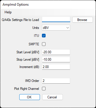
First, let's use the PWR IMD plug-in with the QA40x in single-ended loopback. First, we use ITU-R with an ending amplitude of 0 dBV and focus just on 2nd order products. The setup options are:

And the resulting display is below. Note that our ending level is 0 dBV, and the software has set both the 19 and 20 kHz tones at -3.01 dBV. These sum to give us 0 dBV. Since we're only looking for second order products, the 1 kHz is our sole interest. Some debug code has been added to generate a 3rd sine at 1 kHz and -60 dBV. From the display below, we know the reference level is the sum of the 19 + 20 kHz tones (and that is 0 dBV) and the sole product is at -60 dBV. And so the IMD should be reported as -60 dBC.

The plot below shows the final point at -60 dB, which is correct. Additionally, the 0 dBV = 1Vrms and 8 ohm load equates to 125 mW, which is correct.

Now let's repeat the experiment for 3rd order IMD products. From above, this means we'll look at the sum of the 1k and 18k mixing products. These are of different orders, and so these will be RMS summed. We've again synthesized the additional tones and the plot is as follows. Note that we have both 1k and 18k tones at -60, and the RMS sum of these will be -60 + 3.01 = 56.99 dBV.

And we know our reference level is 0 dBV and the amplitude of the mixing products is -57. And so we expect the reported IMD level to be -57 dBC. That is confirmed by the plot below:

SMPTE

SMPTE is a bit more interesting, because we have pairs of harmonics in-band. Let's first just look at 2nd order harmonics. For SMPTE, that means 6940 and 7060 Hz.

For this, we use the following options. Note we've selected SMPTE, and we've opted for a 2 dBV level.

The resulting plot is as follows. Since the 7 kHz is specified at 12 dB below the specified level, we'd expect the 7 kHz to be at -10 (which it is). We can see the generated products at +/- 60 Hz off the 7 kHz, and we've set each to -60. We can manually compute the IMD. First, we know the IMD reference is the 7 kHz amplitude, which is in this case is -10. Our mixing products can be linearly summed, giving us -54 dBV. And relative to the -10, that gives us a IMD performance of -44 dBc

The graph confirms the math:

Now, let's repeat looking at 3rd order products. Those will be 6880, 6940, 7060 and 7120 Hz. We'll linearly sum the 6880 and 7120 levels, and then linearly sum the 6940 and 7060 levels, and then RMS sum those two results. The plot is below. Again, the reference level is -10. The first products sum to -54, and the second products sum to -54. And the RMS sum of -54 dB and -54 dB will be -51 (all round numbers).

And relative to the -10 reference level, that is -41 dBc which is confirmed by the graph:

Finally, we validate power. We know the 7 kHz tone is at -10, which according to the spec means the 60 Hz tone is at 2 dBV. The total RMS across the 20 kHz measurement is reported at 2.26 dBV = 1.297V, and 1.297^2 / 8 = 210 mW which is also confirmed on the graph above.

IMD with a Class D Amp

Class D amps have a difficult time with the ITU IMD test. As an example, take a look at the plot below. Note that the 19 and 20 kHz tone are likely inaudible to anyone over the age of 12. And yet, a 1 kHz tone has been synthesized by the amp non-linearity. If you listed carefully to this amp through speakers, you'd clearly hear the spurious 1 kHz tone.