Frequency Response with Long Path Delays - QuantAsylum/QA40x GitHub Wiki

Most DUT measurements involve very small path delays. That is, the processing time for the signal inside the DUT is under a millisecond or so. If the circuit is purely analog, then the path delay of the DUT will be measured in microseconds. But if a DSP is involved and perhaps a radio link (such as Bluetooth), the path delay can be 10's of milliseconds. And with some devices, such as effects processors for vocals or guitars, the path delay can intentionally be 100 ms or so (so-called "slap-back" echo). But it isn't uncommon for delays to stretch even longer. Think of a David Gilmore guitar tone, for example, with multiple long-delays cascading over a second.

Release 1.166 of the QA40x software will make it easier to characterize the frequency response of DUTs with long path delays. To examine the changes, we'll start with a guitar effects processor with a delay value set to 100 mS, 100% wet and no feedback. The signal must be 100% wet (delayed signal only) otherwise we're dealing with two signals (dry and wet) at the same time and the result won't make any sense. And delay feedback must be eliminated because, again, if not, we're dealing with more than one signal.

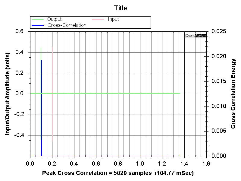
With the QA40x output running to the effect (DUT) input, and the DUT output running to the QA40x input, we can measure path delay (Automated Tests -> MISC Path Delay). The Path Delay plug-in reports 104.77 mS of delay, which is very close to the requested value of 100 mS.

Let's now run a frequency sweep. First, let's do a File->New Settings to put the analyzer into a known state. We can then press the Frequency Response button. And then right click on the FR button and set the amplitude to -20 dBV.

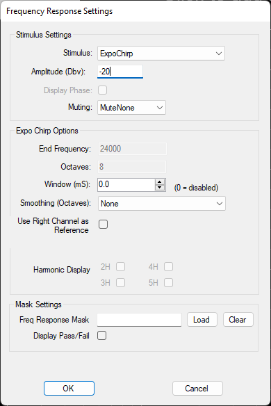
Then click RUN and you can observe the spectrum below.

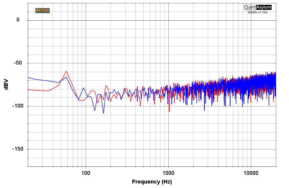
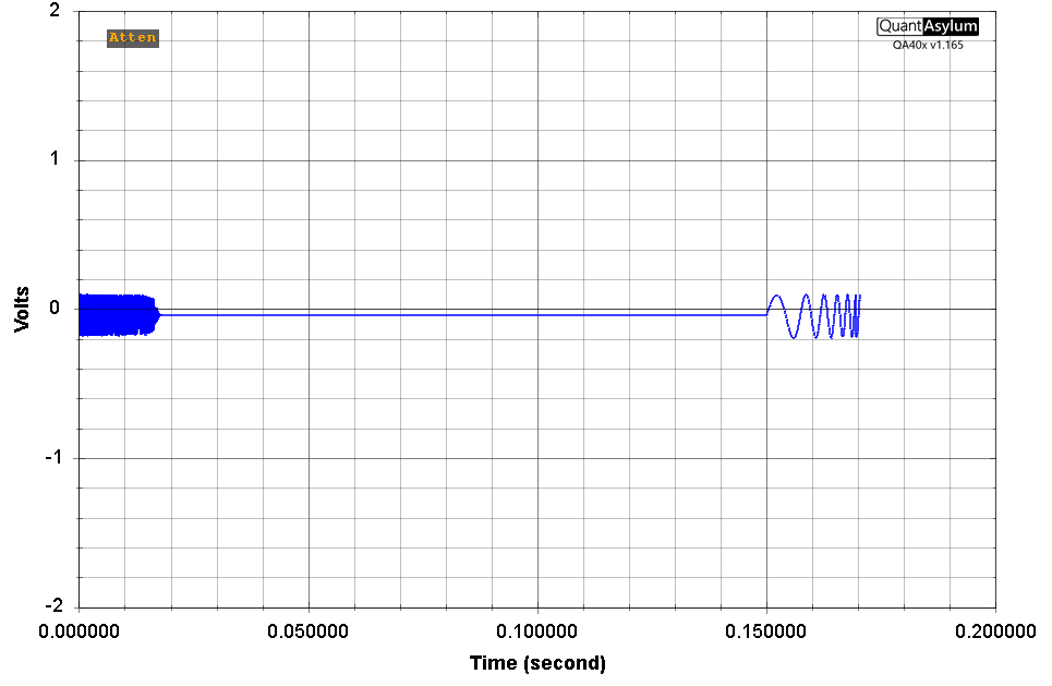
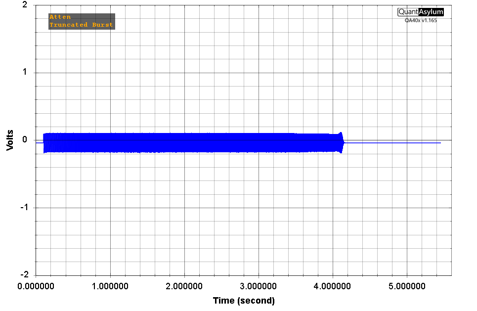
This is very unexpected. What is going on? The clue comes if we look at the time domain (click TIME in the display control block). In the plot below, we can see the low-frequency sweep started on far right side of the display, and wrapped around to the left side. What we're actually seeing here is two different bursts, misplaced in the buffer due to the long delay.

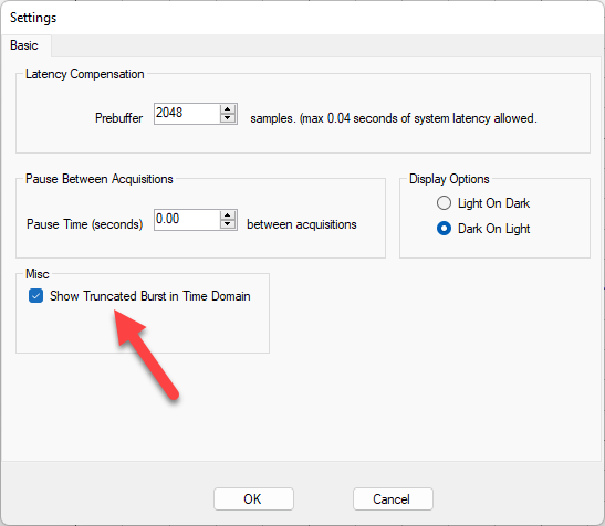
To help sort this out, first go into the Edit->Settings menu and click the Show Truncated Burst in Time Domain. What this does is shows you only the data that is used for the FFT calculations. The pre- and post-buffer regions aren't shown

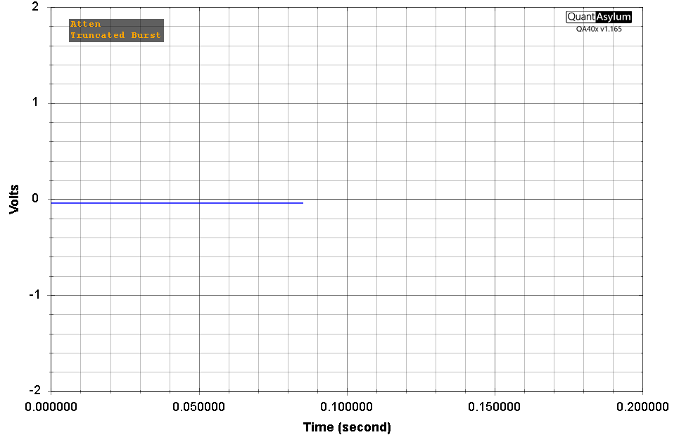
Now, return to the input time domain display. Here we see see the capture buffer is a flat line. Which explain what we saw above where the FR was reported as noise.

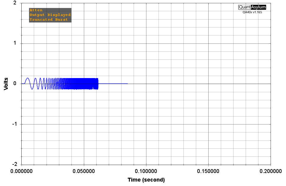
OK, now click the OUTPUT button in the Display control block. Now we're looking at the output buffer in the Time Domain. And this should make sense. We can see the buffer spans from 0 seconds to about 80mS, and place in the middle of the buffer is the chirp.

So what is happening? We know the buffer length is 75 mS, and we know our delay is 100 mS. So, by the time the QA40x outputs the buffer and captures the input, the original signal still hasn't made its way through the delay.

We know that increasing the FFT will increase the length of the buffer. Above, we're using a 4K FFT, which at 48kSps yields 4/48 = 83 mS of buffer. If we grow the FFT to 256K, that will give us a 256/48 = 5.33 seconds of buffer. The plot below shows that. We see the total input signal capture is 5.33 seconds, and we see the recovered signal starts at about 100 mS.

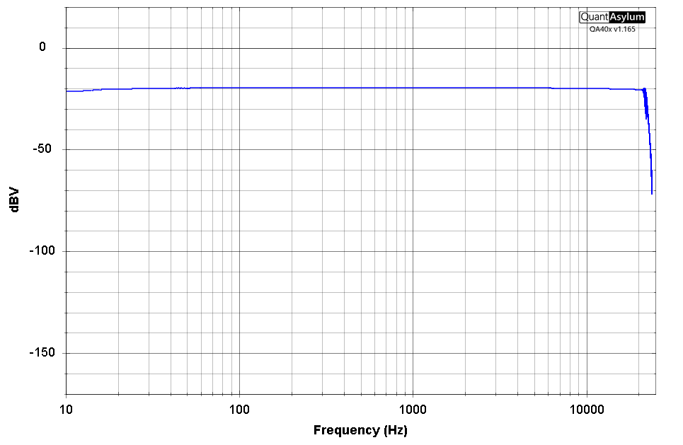
And the resulting frequency plot makes sense:

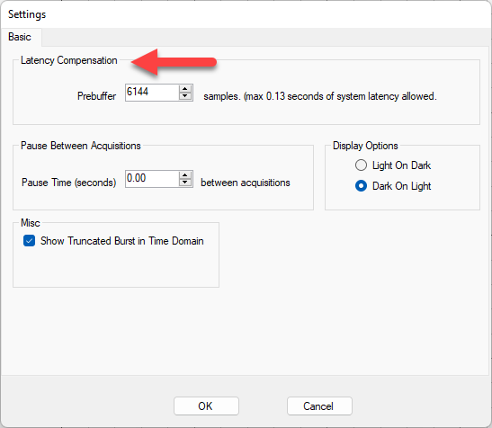
The other way to accomplish this measurement is to use Latency Compensation. When Latency Compensation is set to a number other than the minimum default of 2048, the Frequency Response operates differently. In this mode, the overall buffer size is increased to accommodate the additional path delay that was requested, and the incoming signal is recovered and placed precisely inside the FFT buffer.

In the Settings below, we can see that the prebuffer was increased to 6144 samples, and that it's reported this allows us to deal with 0.13 seconds of latency.

Running a 64K FFT yields the following captured sweep in the time domain:

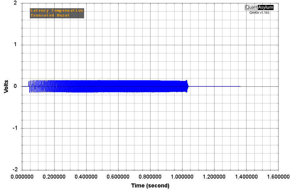
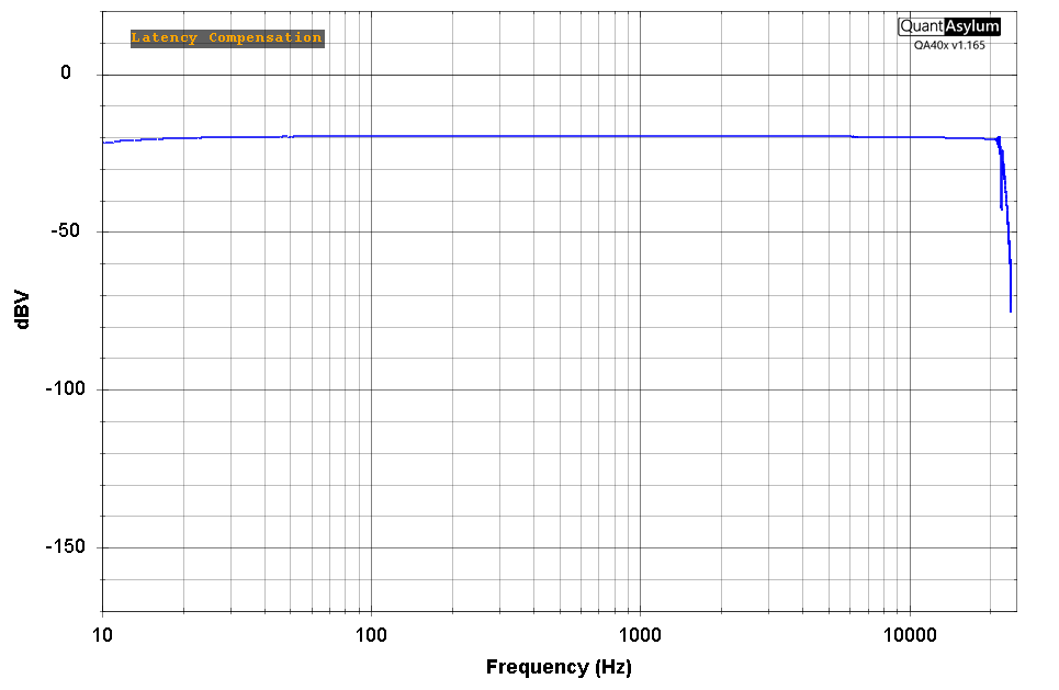
Note that above this full chirp is inside the buffer--the Truncated Burst annunciator indicates this is the actual buffer. And the Latency Compensation annunciator while using chirps indicates that additional work is being done to locate the chirp in the buffer. In other words, a what we're seeing in the buffers isn't what has actually occurred--it's been "helped" into place by the software.

And the resulting frequency response plot of the 100 mS delay is shown below: