LCA CIFAR Tutorial Part1 One Image - PetaVision/OpenPV GitHub Wiki
In this part of the tutorial, you will use PetaVision and the LCA to create a sparse encoding of a single image, and to retrieve the information in the files generated by the PetaVision run. This page uses Python 3 to analyze the PetaVision output. If you would prefer to use GNU Octave for the analysis, please see this page.
This tutorial assumes you have OpenPV and all dependencies downloaded and built with the CUDA, cuDNN, and OpenMP flags on. For further information on installation, please refer to:

Natural scenes can be decomposed into basic image primitives using sparse coding [Olshausen and Field, 1996]. A patch of an image can be represented as a linear sum of feature vectors {ɸi}, weighted by coefficients {ai}. When the number of feature vectors is greater than the number of pixels in the patch to be reconstructed, there in general exists an infinite number of ways (linear combinations) to reconstruct the patch. However, sparse coding aims to select a particular linear combination that minimizes the number of feature vectors with nonzero weights. The sparse code itself minimizes an energy function that balances the number of active elements with reconstruction fidelity.
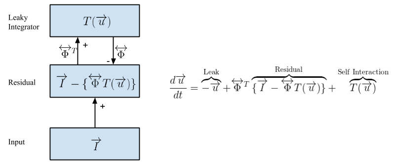
Here, we will use OpenPV to sparse code images using the Locally Competitive Algorithm (LCA) [Rozell et al., 2008]. LCA is shown schematically in the figure above. In LCA, the coefficients {ai} are determined by a set of membrane potentials {ui}, through a transfer function a = T(u). Here, the transfer function T(u) depends on a threshold λ, and T(u) = 0 for |u| < λ.
At the center of our LCA implementation is the Residual layer, which computes the difference between the input image I and the sparse reconstruction of that image, given by a linear combination of features weighted by activation coefficients T(u)ɸ. The neurons that generate the sparse code are located in a Leaky Integrator layer. Activity in the leaky integrator is not driven by the inner product of the feature vector and the image I, as in most neural networks; but rather by the inner product of the feature vector and the the Residual layer. Because activity is driven by the instantaneous image reconstruction error, this creates lateral competition between the leaky integrator neurons, since any pixels explained by a particular leaky integrator neuron are unavailable to drive activity in the other leaky integrator neurons. A self-interaction ensures that individual leaky integrator neurons don't compete with themselves. It can be shown mathematically that the above model converges to a sparse representation of the input image I. This tutorial aims to provide an intuitive sense of LCA through a hands-on demonstration. One advantage of LCA is that it is very parallelizable, allowing for the use of GPUs or neuromorphic hardware.
These tutorials use /path/to/source/OpenPV as the path to the OpenPV source
directory, and /path/to/build-OpenPV as the path to the build directory.
Replace these paths with the paths you have on your system.
First, navigate to the build directory. Then create an LCA-CIFAR-Tutorial
directory and switch into it.
$ cd /path/to/build-OpenPV # change this path to the correct path on your system
$ mkdir LCA-CIFAR-Tutorial
$ cd LCA-CIFAR-Tutorial
We will need to set the shell environment variable PV_SOURCEDIR to the source
directory when running lua, and it will be convenient to use this environmental
variable at other times as well.
$ PV_SOURCEDIR=/path/to/source/OpenPV # change to the correct path on your system
$ export PV_SOURCEDIR
Next, download the python version of the CIFAR dataset from the CIFAR website and move the .tar.gz into the current directory. This can be done using the following wget command in the terminal.
$ wget "https://www.cs.toronto.edu/~kriz/cifar-10-python.tar.gz"To extract the CIFAR-10 dataset into PNG files, run the following script in the source directory. The script depends on the imageio and numpy python packages.
$ python $PV_SOURCEDIR/tutorials/LCA-CIFAR/scripts/extract_cifar.pyThis script creates a directory named cifar-10-images. Within that directory
are ten subfolders named 0 through 9. These subfolders correspond to the ten
CIFAR-10 categories. In each subfolder are 6000 32x32x3 PNG files. There are
also text files listing the images from each data batch and from the test batch.
Finally, the mixed_cifar.txt file contains all of the data_batch images but
not the test images. This page will perform a run on one of the images; later
in the tutorial we will do runs with multiple images.
The parameters for our run are defined in a Lua script; it is in the source
directory at the path $PV_SOURCEDIR/tutorials/LCA-CIFAR/input/LCA_CIFAR.lua.
Over the course of the tutorial we will modify the Lua input; hence it is
convenient to copy input directory from the source tree to the build tree, and
do the modifications on the copy.
$ cp -r $PV_SOURCEDIR/tutorials/LCA-CIFAR/input input
$ ls input
LCA_CIFAR_full.lua LCA_CIFAR.lua  LCA_CIFAR.png
We will be using the LCA_CIFAR.lua file. The most relevant parameters of the model are set at the top of this file, with documentation on what each parameter does. The rest of these parameters are already tuned for this tutorial.
To find PetaVision-specific Lua modules, the Lua script reads the environment
variable PV_SOURCEDIR (which we set above) for the OpenPV source directory.
If this variable is not set, it uses $HOME/OpenPV as the default.
The .lua file assumes that you compiled with CUDA/cuDNN and are on a machine with a GPU. If you compiled without CUDA, edit the LCA_CIFAR.lua file to change the line
local useGpu = true;
to
local useGpu = false;
The output of the Lua script is a text file of parameters which PetaVision will
read as its input. The usual filename extension for a parameter file is
.params.
$ lua input/LCA_CIFAR.lua > input/LCA_CIFAR-One-Image.paramsA more detailed description of the .params file will wait until later in the tutorial, but here we provide some general ideas.

The figure above shows the layers of an LCA implementation.
-
Inputtakes an image from the CIFAR-10 dataset, normalizes luminance, and passes its values toInputErroron the positive channel, where the values are simply copied over. -
InputErrorcomputes the difference between the input and the reconstruction fromInputRecon, which drives the minimization of the sparse coding energy function in the leaky integrator, here labeledV1. - The connection from
V1toInputErrorcomputes the reconstructed image from the sparse coding.
After generating the OpenPV parameter file, we can now start the run. Here we use one of the system test executables (BasicSystemTest) to run the model (Later releases will have a dedicated executable).
To run the network, make sure you are still in the LCA-CIFAR-Tutorial directory of the build directory, and run the command:
$ ../tests/BasicSystemTest/Release/BasicSystemTest -p input/LCA_CIFAR-One-Image.params -l LCA-CIFAR-run.log -t 2The arguments and their meanings are as follows.
| Run-time flag | Description |
|---|---|
| -p /path/to/pv.params | Use this path for the parameters file (required) |
| -l /path/to/log.txt | Write a log file to this path (if absent, log messages will be written to stdout or stderr) |
| -t number | Use this many OpenMP threads (required if compiled with OpenMP) |
OpenPV writes its output to binary '.pvp' files, and the output of probes to text files. OpenPV includes a python package for reading .pvp files and probe output into python numpy arrays.
The PetaVision run creates an output directory specified by the outputPath lua variable. It also generates a .log file at the path given in the -l option.
The output directory contains several output files and a Checkpoints folder.
| File or Folder/ | Description |
|---|---|
*.pvp |
All groups of the parameter file that have a writestep ≥ 0 write output to a pvp file. |
AdaptiveTimescales*.txt |
Record of Error layer timescales |
Checkpoints |
Periodic snapshots of the run |
CIFAR_Tutorial.params |
OpenPV-generated params file; includes defaults, omits unnecessary params; removes comments |
CIFAR_Tutorial.params.lua |
OpenPV-generated base lua file. |
InputErrorL2Norm*.txt |
L2 norm of reconstruction error |
NumNonzeroProbe*.txt |
L0 norm (number of nonzero values) of the leaky integrator layer |
SparsityProbe*.txt |
Sparsity penalty of the sparse coding leaky integrator layer |
timestamps/Input.txt |
Files generated from the ImageLayer to specify which image was read at which simulation time. |
TotalEnergyProbe*.txt |
Total values of the objective function that LCA minimizes |
Depending on the size of a run and how frequently you set the writeStep parameter, the size of your .pvp files can range from KB to GB. For this (short) run, the input, error, and recon layers have .pvp files of about 5MB, and the LeakyIntegrator layer is about 14MB. The LeakyIntegratorToInputError .pvp file is about 40MB.
We provide basic tools for reading various types of .pvp files into a Python numpy array. We will be using the numpy and matplotlib packages, as well as the pvtools package in the source directory's python folder. Internally the pvtools package depends on the scipy package. To find the pvtools package, python needs to have the the directory it's in added to the PYTHONPATH environment variable. Be sure to replace "/path/to/source/OpenPV" with the path to the OpenPV repository on your system. Set PYTHONPATH, and then start python.
$ export PYTHONPATH="$PYTHONPATH":$PV_SOURCEDIR/python
$ pythonAs a simple analysis case, let's view an original image and its reconstruction.
>>> import pvtools

>>> input_data = pvtools.readpvpfile("output/Input.pvp")
>>> recon_data = pvtools.readpvpfile("output/InputRecon.pvp")
The readpvpfile() function loads the .pvp file into a dictionary with keys
header, values, and time. If we take a look at the header, we can find
various information about the file that is useful for analysis scripts.
>>> input_header = input_data['header']
>>> for k in input_header.keys():
...   print(f'{k:10} = {input_header[k]}')
...
headersize = 80
numparams  = 20
filetype   = 4
nx         = 32
ny         = 32
nf         = 3
numrecords = 1
recordsize = 3072
datasize   = 4
datatype   = 3
nxprocs    = 1
nyprocs    = 1
nxExtended = 32
nyExtended = 32
kx0        = 0
ky0        = 0
nbatch     = 1
nbands     = 401
time       = 0.0
Next, let's take a look at the data structure.
>>> input_values = input_data['values']
>>> input_values.shape
(401, 32, 32, 3)
There are 401 frames in the data structure, corresponding to the initial time t=0 and the 400 timesteps of the run. This number agrees with the nbands field of the header. Each frame is 32-by-32 with three features, corresponding to the size of the CIFAR-10 images, which are 32-by-32 images with three color channels. These values appear in the header as the nx, ny, and nf fields.
Finally, the time field contains the simulation time at which each of the
frames were written.
>>> input_times = input_data['time']
>>> input_times.shape
(401,)

>>> input_times
array([  0.,   1.,   2.,   3.,   4.,   5.,   6.,   7.,   8.,   9.,  10.,
        11.,  12.,  13.,  14.,  15.,  16.,  17.,  18.,  19.,  20.,  21.,
        22.,  23.,  24.,  25.,  26.,  27.,  28.,  29.,  30.,  31.,  32.,
[...]
       385., 386., 387., 388., 389., 390., 391., 392., 393., 394., 395.,
       396., 397., 398., 399., 400.])
The length of the time array is the number of frames, and each value gives the simulation time when that frame was written. In this case, frame n is written at time t=n (the frames are zero-indexed and the inital data at t=0 is included).
Let's see what the image and reconstruction look like at the initial time.
>>> input_frame = input_values[0]

>>> recon_values = recon_data['values']
>>> recon_frame = recon_values[0]

>>> import numpy
>>> concatenated = numpy.vstack([input_frame, recon_frame])
The input images, as written to the output directory, are normalized: for each image, the pixel values have zero mean and unit standard deviation. We rescale to the range 0-255 and display.
>>> concat_normalized = (concatenated - numpy.min(concatenated)) / (numpy.max(concatenated) - numpy.min(concatenated))
>>> concat_8bit = numpy.uint8(concat_normalized * 255)

>>> import matplotlib.pyplot
>>> matplotlib.interactive(True)
>>> matplotlib.pyplot.figure(1)
>>> matplotlib.pyplot.imshow(concat_8bit)
The CIFAR-10 image being processed, at top, is one of the images in the frog category. The reconstruction is initially blank.
Let's see how the reconstruction looked at the end of the run.
>>> input_frame = input_values[400]
>>> recon_frame = recon_values[400]
>>> concatenated = numpy.vstack([input_frame, recon_frame])
>>> concat_normalized = (concatenated - numpy.min(concatenated)) / (numpy.max(concatenated) - numpy.min(concatenated))
>>> concat_8bit = numpy.uint8(concat_normalized * 255)
>>> matplotlib.pyplot.imshow(concat_8bit)
As you should be able to see, the reconstruction looks similar to the original image, but the error is quite noticeable, as the run has not learned weights suitable to the dataset.
The dictionary of features is in the connection "LeakyIntegratorToInputError"
and the evolution of the dictionary is written to the
output/LeakyIntegratorToInputError.pvp file. Let's see how the weights
are stored.
>>> weights_data = pvtools.readpvpfile("output/LeakyIntegratorToInputError.pvp")
>>> weights_header = weights_data['header']

>>> for k in weights_header.keys():
...   print(f'{k:10} = {weights_header[k]}')

headersize = 104
numparams  = 26
filetype   = 5
nx         = 1
ny         = 1
nf         = 128
numrecords = 1
recordsize = 0
datasize   = 4
datatype   = 3
nxprocs    = 1
nyprocs    = 1
nxExtended = 1
nyExtended = 1
kx0        = 0
ky0        = 0
nbatch     = 1
nbands     = 1
time       = 0.0
nxp        = 8
nyp        = 8
nfp        = 3
wMin       = -0.6359400153160095
wMax       = 0.5457189679145813
numpatches = 128
The weights header contains all the same fields as the layer header, plus
several additional fields. However many of the fields are no longer used and
are still present only for reasons of backward compatibility. Of interest to us
are nx = 8, ny = 8, nf = 3, and numpatches = 128. They tell us that
the dictionary elements are 8x8x3 pixels each, and that the dictionary has
128 elements.
>>> weights_data['time']
array([0.])
Here the time field only contains a single element, because we only wrote the weights once, at the beginning of the run. We are not yet learning the weights, so there is no need to write the weights more than once. In the lua file, the first time the weights are written is specified by the connInitialWrite variable, and the period is specified by connWriteStep. Here connInitialWrite is set to 0, and connWriteStep is set to infinity. Later in the tutorial, when we introduce learning weights, we will change the value of connWriteStep.
>>> weights_values = weights_data['values']
>>> weights_values.shape
(1, 1, 128, 8, 8, 3)
The first dimension, 1, is the number of times at which the weights were written, as described above. The second dimension, 1, indicates the number of axonal arbors; in this tutorial we are only using a single arbor. The third dimension, 128, is the number of dictionary features, and the remaining dimensions, (8, 8, 3), specify the size of each dictionary element.
To display the patches, we will arrange them in a tableau of 11 rows and 12
columns, with 4 spaces left blank. The pvtools function arrangedictionary
arranges them in this manner. It also rescales each feature to the interval
[-1,1].
>>> weights = weights_data['values'][0, 0]
>>> numpy.min(weights)
-0.6359400153160095

>>> numpy.max(weights)
0.5457189679145813

>>> wgts_display = pvtools.arrangedictionary(weights)
>>> wgts_display.shape
(88, 96, 3)

>>> numpy.min(wgts_display)
-1.0

>>> numpy.max(wgts_display)
1.0
In order to display the weights, we convert to 8-bit values.
>>> wgts_display_8bit = numpy.uint8(wgts_display * 127.5 + 127.500001)
>>> matplotlib.pyplot.clf()
>>> matplotlib.pyplot.imshow(wgts_display_8bit)
This shows the initial weights, which are mostly zero with a few nonzero values at random locations. As we saw in the previous section, we can use these weights to sparse code an image, but the sparse coding will not be very good.
As discussed at the beginning of this tutorial, the LCA minimizes an objective
function. The objective function is calculated by a probe, named
TotalEnergyProbe in the params file. The probe produces the
TotalEnergyProbe_batchElement_0.txt text file in the output directory. This
run looked at a single image, so the batch size was 1, and each probe produces
only a single output text file (with index 0).
Let's look at the contents of the probe output file. Exit python for now, or use another terminal window to inspect the file.
$ head output/TotalEnergyProbe_batchElement_0.txt
time,index,energy
  1.000000, 0, 1537.383299127
  2.000000, 0, 1534.488694107
  3.000000, 0, 1531.883096583
  4.000000, 0, 1528.487269416
  5.000000, 0, 1525.028296310
  6.000000, 0, 1521.505614520
  7.000000, 0, 1517.918903758
  8.000000, 0, 1514.267251211
  9.000000, 0, 1510.550653218

$ tail output/TotalEnergyProbe_batchElement_0.txt
391.000000, 0, 778.535635298
392.000000, 0, 778.513739818
393.000000, 0, 778.493150292
394.000000, 0, 778.473222118
395.000000, 0, 778.452910503
396.000000, 0, 778.432210680
397.000000, 0, 778.410978743
398.000000, 0, 778.389987279
399.000000, 0, 778.369409432
400.000000, 0, 778.348745163
(Your results may differ in the last few decimal points).
The file consists of a header row, listing the fields time, index, and energy. The time field gives the timestep. In this case it ranges from 1 to 400, since the run went for 400 timesteps. The index field is the batch element's index, it is always the same within each individual probe output file. The third field, energy, is the value of the objective function being minimized. We can see from the above output that the energy is decreasing over the run, and the decrease is much slower at the end of the run than the beginning.
Let's load all the data into python and plot the energy values over the entire run.
$ python
>>> import numpy
>>> probedata = numpy.loadtxt('output/TotalEnergyProbe_batchElement_0.txt', delimiter=',', skiprows=1)
>>> probedata.shape
(400, 3)
>>> timestamps = probedata[:, 0]
>>> energy = probedata[:, 2]

>>> import matplotlib.pyplot
>>> matplotlib.interactive(True)
>>> matplotlib.pyplot.plot(timestamps, energy)
>>> matplotlib.pyplot.plot('Total Energy')
The plot shows that the energy starts at about 1500, and then decreases steadily over the run, appearing to converge to a new steady state of about 800 by approximately t=200.
There is a function readenergyprobe in the pvtools package, that reads an
energy probe. We can recreate the above plot using that function:
>>> import pvtools
>>> energydata = pvtools.readenergyprobe(
...   probe_name='TotalEnergyProbe',
...   directory='output',
...   batch_element=0)
>>> matplotlib.pyplot.figure(2)
>>> matplotlib.pyplot.plot(energydata['time'], energydata['values'])
>>> matplotlib.pyplot.plot('Total Energy')The objective function consists of a sum of two terms, each consisting of a
norm of one of the layers: the L1 norm of the LeakyIntegrator layer, and the
L2 norm of the residual layer InputError. These norms are computed by layer
probes named SparsityProbe and InputErrorL2NormProbe, respectively. They
write text output, with filenames constructed the same way as the energy
probes.
The layer probe output files have a different format from those of energy probes. There is no header line, and the lines contain four fields. These fields are the timestamp, the batch element, the number of neurons in the layer, and the value of the norm. Therefore, they are read using the readlayerprobe function in pvtools.
>>> sparsity = pvtools.readlayerprobe(
...   probe_name='SparsityProbe',
...   directory='output',
...   batch_element=0)
>>> sparsity['values'].shape
(401, 1)
>>> inputErrorL2Norm = pvtools.readlayerprobe(
...   probe_name='InputErrorL2NormProbe',
...   directory='output',
...   batch_element=0)
>>> inputErrorL2Norm['values'].shape
(401, 1)
Note that the layer probe's data is one row longer than the energy probe's. This is because layer probes output the value at time zero, but energy probes only start at time t=1. We can see how each of the layer probes evolves over the run.
>>> matplotlib.pyplot.figure(1)
>>> matplotlib.pyplot.clf()
>>> matplotlib.pyplot.plot(
...   sparsity['time'], sparsity['values'])
>>> matplotlib.pyplot.title('Leaky Integrator L1-norm')

>>> matplotlib.pyplot.figure(2)
>>> matplotlib.pyplot.clf()
>>> matplotlib.pyplot.plot(
...   inputErrorL2Norm['time'], inputErrorL2Norm['values'])
>>> matplotlib.pyplot.title('Input Reconstruction Error L2-norm')
At the start of the run, the leaky integrator layer has no activations. Hence the sparsity penalty measured by SparsityProbe is zero. However, the reconstruction error is large because the reconstructed image is all zero. As the LCA progresses, the leaky integrator layer activates neurons that reduce the reconstruction error. As it does so, the InputErrorL2Norm decreases and the sparsity penalty increases, eventually converging to some steady state. The reconstruction error does not become zero, however, because achieving a perfect reconstruction would require too many active dictionary elements, and therefore cause a large sparsity penalty.
The total energy is given by
E = λ * sparsity['values'] + (1/2) * inputErrorL2Norm['values']
where λ is the threshold of the transfer function. It appears in the .lua and .params files as VThresh. For this run, λ = 0.55.
The (1/2) is the usual coefficient multiplying the square of an L2-norm. It is set by the coefficient field in the InputErrorL2NormEnergy group near the bottom of the lua file. However, this parameter is typically not changed.
You can compare the values of energydata to result the of this expression. They should match up to floating-point accuracy. Remember that the times for the energy probe start at t=1 and the times for layer probes start at t=0. We'll plot each term of the expression for E, together with the total E, on the same plot.
>>> matplotlib.pyplot.figure()
>>> matplotlib.pyplot.clf()
>>> matplotlib.pyplot.plot(energydata['time'], energydata['values'])
>>> matplotlib.pyplot.plot(sparsity['time'], 0.55 * sparsity['values'])
>>> matplotlib.pyplot.plot(
...   inputErrorL2Norm['time'], 0.50 * inputErrorL2Norm['values'])
>>> matplotlib.pyplot.title('Components of Total Energy')
The sparsity penalty in this run uses the L1 norm. In some cases, we might be
more interested in the L0 norm, that is, the number of neurons with nonzero
activity. The .lua file adds one more layer probe to LeakyIntegrator,
NumNonzeroProbe which counts the number of leaky integrator neurons with
nonzero activity at each timestep. This probe is not included in the
calculation of total energy for this run, but can still give useful
information.
>>> matplotlib.pyplot.figure()
>>> numNonzero = pvtools.readlayerprobe(
...   probe_name='NumNonzeroProbe',
...   directory='output',
...   batch_element=0)
>>> matplotlib.pyplot.plot(
...   numNonzero['time'], numNonzero['values'])
>>> matplotlib.pyplot.title('Leaky Integrator L0-norm')We can see the evolution of the reconstruction using the animate_layers.py
script. Exit Python and run the following command:
python $PV_SOURCEDIR/tutorials/LCA-CIFAR/scripts/animate_layers.py output/Input.pvp output/InputRecon.pvp recon.gifOpening the recon.gif file will show the recon layer evolving from flat gray to a close approximation of the original image.
In this page, we saw how to use PetaVision to sparse code an image using random initial weights. In the next part of the tutorial, we will see how PetaVision implements parallelism to process multiple images.