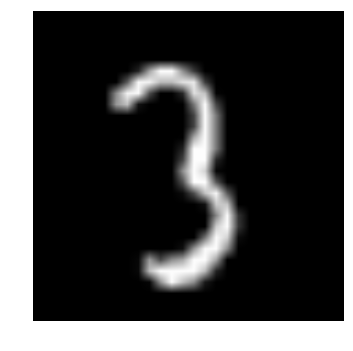
In this example, we are trying to recognize which digit is present in a 28x28 pixel greyscale image. Here's an example of one of the images:

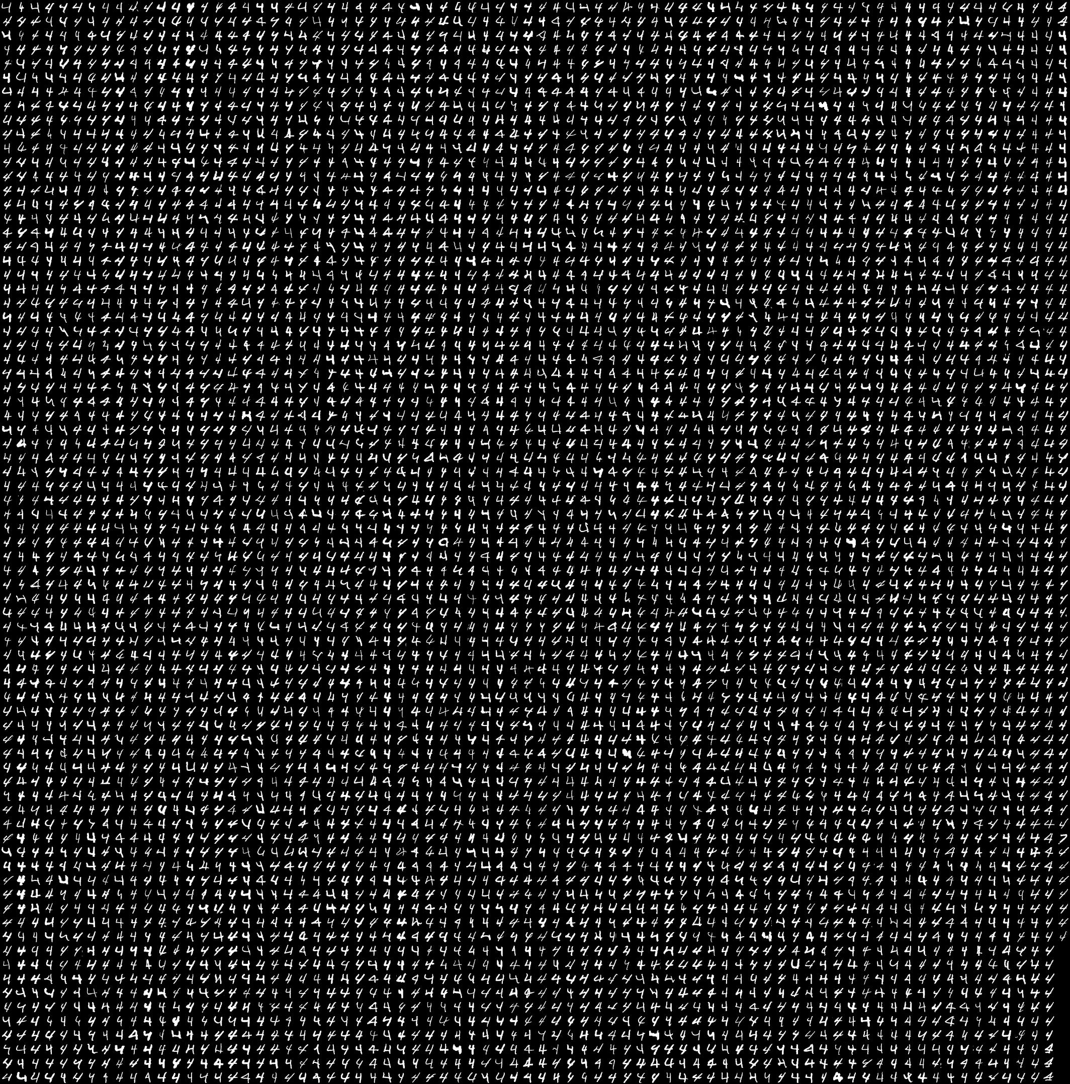
The MNIST dataset has a large collection of images, each labeled with the correct digit displayed in that image. Using this information we can 'train' our network to recognize each of the ten 'classes,' one for each digit. Every image will be labeled 0-9. Note that the images in the dataset contain a lot of variation, as you would expect from handwritten characters. Here's an example of several different '4's in the dataset:

We will be using Python, TensorFlow, and TFLearn to write our code. If you havn't done so already, follow the getting started guide Once you're all setup, let's write some code!.

Python is a dynamically typed language, meaning that there is no distinction between int variables, String variables, floats and so on. They are all just variables. The syntax of Python is relatively simple, with the only complication being that whitespace matters. In Python, indenting your code properly is not just a good practice, it is part of the language syntax.

Python by default comes with an interpreter that can be used on the command line. Run python3 with no parameters, and you will be given an interactive shell where you can type Python code, and it will be executed on the fly. This removes the need for a separate compiler.

To run python scripts that you write, run python3 myScript.py. Lines in the script file are executed from top to bottom - there is no notion of a 'main' function or entry point to your code. Any and all lines in the file are

Variables do not need to be declared, unlike in C or Java (ex: int myVar;) So this is perfectly fine before declaring anything:

myvar = 20

Variables have no type, so this is perfectly OK:

myVarl = 20
myVar1 = "yes"

We can even compare and attempt to combine different types, with varying degrees of success.

print("yes" == 20)
print("yes" * 10)

Also, the print() statement is nothing like the old printf() commands or System.out.println() in Java. It's much better and more flexible. It takes arbitrary types and any amount of arguments. For instance:

print("Hello World!", 20, True)

uses three arguments of different types, and is perfectly OK.

if statements, while similar to C/Java, have a different syntax, but do the same thing. Note that indentation is critical here:

if myVar==20:
  print("omg, the variable is", myVar)
else:
  print(myVar, "is not 20.")
  myVar = myVar + 1   # note, this is a comment
  myVar += 5  # or we can add something other than 1
print("This is not part of the if clause")

Functions can be declared anywhere in the file, even inside other functions! The syntax is different from C/Java yet again, and also note that we don't have to define what types our arguments are. Note again that indentation is critical, as it determines what is and what is not part of the function definition.

def myNewFunction(name, date):
  print("Hello", name)
  print("The date is", date)

myNewFunction("Bob", "2/12/17")

TensorFlow is a Python library for writing computational code with large dimensional data, and distributing the computation across several computers or processors efficiently. It also happens to be very good for neural networks and machine learning because of this. After all, most machine learning algorithms are just computations with high dimensional data. TensorFlow automatically does things like calculate derivatives of computations, has many built in functions for neural networks and has been geared towards that use case.

TFLearn makes using TensorFlow for neural networks and machine learning easy. TensorFlow by itself is extremely powerful and flexible. However, using that power takes some knowledge and experience. TFLearn, by comparison, can be used and understood by just about anyone in, say, a three-hour session.

In order to use libraries in python, you need to import them, just as with C/Java. In Python, this looks like:

import tflearn

However, there are lots of options available to us as well. For instance, we can load just a part of a library:

from tflearn import datasets

which will only import the datasets module.

There's also

import tflearn as tf

which we will see later allows us to access TensorFlow through a new name, tf, rather than spelling out tflearn.

• First things first, we need to import the tflearn library, as well as the MNIST dataset we will be using. Fortunately, tflearn already includes this dataset for us.

import tflearn
import tflearn.datasets.mnist as mnist  # name it mnist so we don't need to spell out tflearn.datasets.mnist all the time

The next step is to build our network. It will look something like this:

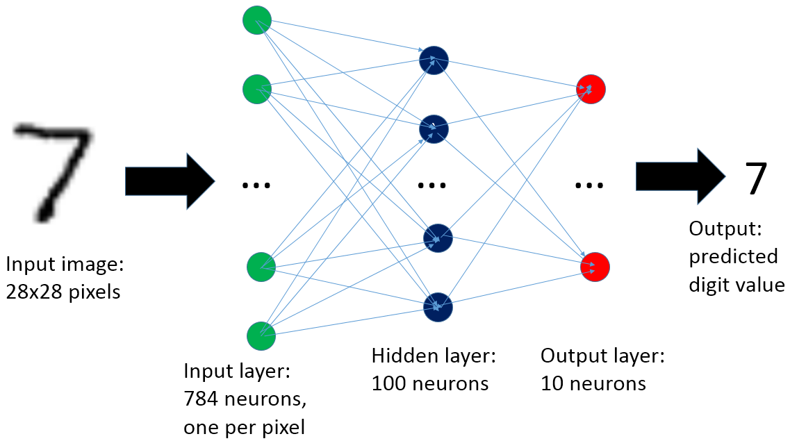
In TFLearn, that means we need 3 layers, an input layer of size 784, a single hidden layer with 100 neurons (size 100), and an output layer with 10 classes (size 10). How the output works is that each node in the output layer acts as a confidence of how much the network thinks the image looks like that particular class. So whichever output node has the largest value is likely the digit that is in the picture.

Note the activation functions for each layer. The tanh function is for the hidden layers, scaling the output to a range of -1 to 1, whereas the output layer uses a softmax function which will normalize all our values to the range 0 to 1, while also making sure that they all add up to one. This lets us use the outputs as a probability distribution where each node is the probability that the image is in a particular class.

# build the network
input_layer = tflearn.input_data(shape=[None, 784])
hidden_layer = tflearn.fully_connected(input_layer, 100, activation='tanh')
output_layer = tflearn.fully_connected(hidden_layer, 10, activation='softmax')

We also need to load our data, however how we load it is important. Note that we are using a probability distribution for our output layer due to the softmax function. Our training examples need to be formatted in a similar way, aka a 10-dimensional vector of probabilities from 0-1 and summing up to one so that we can compare the two later in our loss function. Since we know the digit in the image, we can think of the probability of the image being that digit as 100%, and all other digits as 0%. This format is know as 'one-hot' and TFLearn has a simple helper function to format the data accordingly.

X, Y, testX, testY = mnist.load_data(one_hot=True) # loads the training data, X,Y and the test data testX,testY

Once we have the network, we need to set up how we want to train this network. This is the machine learning step. We will use the SGD (Stochastic Gradient Descent) optimizer. There are other optimizer algorithms that behave slightly differently, but SGD is fairly good, and easy to understand. For our loss function, i.e. how bad is our network doing, we will use the mean squared error from the 'true' value. That means every output node will have an error value that is (real-output)². This error is what is used to adjust the weights so that the node will have less error in the future for that specific data.

A note about the learning rate: When we adjust our weights based on the error, we only know which direction or gradient we should adjust them towards. But how much should we change them? for example, if you were finding the vertex of a parabola, and you knew the derivative was negative, you would know you needed to move to the right to find a lower point on the function. But how far to right should you go? If you go too far, you could miss the vertex. If you don't go far enough, you may take a long time to get there. This notion of 'how far' to change is called the learning rate. Faster learning rates will adjust the weights faster, but may easily skip over any local min/max in the function that we are trying to find. This means that our network will never be very good. If the learning rate is too slow, it takes too long to train. To mitigate this slightly, and prevent oscillating around the min/max point, we use a learning rate decay, meaning that over time, the learning rate decreases, so that we converge to the true solution.

(red showing large fixed learning rate, green showing smaller, decaying learning rate)

# Regression using SGD with learning rate decay
# Create the optimizer function
sgd = tflearn.SGD(learning_rate=0.1, lr_decay=0.96, decay_step=1000)
# Create a function to define our model's accuracy. (use tflearn's built-in)
accuracy = tflearn.metrics.Accuracy()
trainer = tflearn.regression(output_layer, optimizer=sgd, loss='mean_square', metric=accuracy)

And finally, we can train the network on the data using TFLearn's built in functions

# Training
model = tflearn.DNN(output_layer, tensorboard_verbose=0)
model.fit(X, Y, n_epoch=20, validation_set=(testX, testY), show_metric=True)