RFC 20121122: Partial Vaccine Immunity - NAVADMC/ADSM GitHub Wiki

Applies to: Model description v1.0.0

Type of change: New feature, for next minor revision of the software.

Summary: This RFC adds variable levels of vaccine immunity.

Justification: The existing vaccination model does not capture vaccination of only some animals in a unit, or vaccine efficacy.

#Background

ADSM is herd-level with the possible states being: Susceptible, Latent, Subclinical Infectious, Clinical Infectious, Naturally Immune, Vaccine Immune, and Destroyed.

The states are not completely all-or-nothing: there is a “prevalence curve” overlaid during the Latent, Subclinical Infectious, and Clinical Infectious states to express the prevalence of infected animals within the unit.

ADSM takes an all-or-nothing approach to vaccination:

• When a unit is vaccinated, there is a delay for immunity to develop.
• If the unit receives an effective exposure during this delay period, the unit becomes infected and the vaccine has no effect.
• Once immunity has developed, the unit is 100% protected against subsequent exposures.
• If an already-infected unit is vaccinated, the vaccination has no effect.

Problem statement:

The modeling group wants to explore the effects of varying:

• The proportion of animals within a unit that are vaccinated
• The vaccine efficacy.

For ease-of-use, the modeler should enter these values — proportion of animals vaccinated, vaccine efficacy — directly, since these represent concrete real-world numbers. The challenge is to translate those numbers, in some biologically justified way, into effects in the herd-level model.

Concept:

Can a mathematical formula be found that describes how to transform the existing prevalence curve in two situations:

• a unit is vaccinated when it was already infected x days ago
• a unit is infected when it was already vaccinated y days ago

The transformation might for example be specified in terms of shifting the prevalence curve along the days axis, lengthening the curve along the days axis, or flattening the curve along the prevalence axis.

#Experiment 1

In the February 2013 meeting in Fort Collins, it was suggested to use the within-herd disease progression model developed for NAADSM v5 to explore the effects of vaccinating at different levels of coverage and at different times relative to the effective exposure. The research question was to see if those numbers translate predictably into shifting, lengthening, or flattening of the prevalence curve.

##Experiment 1 setup

Within-herd parameters were taken from a document written by G. Garner in which he was preparing prevalence parameters for the QUADS comparison exercise.

• Number of animals: 293
• Latent period: 4 days
• Infectious clinical period: 6 days
• Daily adequate contact rate: triangular distribution 1.1 - 1.4 - 2.2
• Uniform mixing
• Natural immunity period (after transition from infectious): forever (365)
• Delay to vaccine immunity: uniform distribution 3 - 5
• Vaccine immunity period: triangular distribution 21 - 28 - 35

(Latent, immune, etc. period are all animal-level.)

The population contains 2 units, A and B. A is the unit whose states will be tracked. B is initially infected; its role is to create an adequate exposure to A and/or get detected and initiate vaccination.

To create a scenario where vaccination happens before infection,

• NAADSM 5’s routine vaccination module is used to put unit A in a vaccine immune state at the start of the simulation, with a given percentage of animals vaccinated.
• the latent period of unit B is varied to delay the adequate exposure from B→A until a given day.

To create a scenario where infection happens before vaccination,

• A starts out susceptible.
• There is an adequate exposure from B→A on the first day of the simulation.
• B is detected on the first day of the simulation, which creates a request to vaccinate A.
• The day on which vaccination capacity becomes available is varied to delay the vaccination until a given day.

80% vaccination was used because 80% has been mentioned as the coverage that achieves herd-level immunity. (Here, 80% is the percentage of animals who become vaccine immune assuming there is no infection in the scenario. It is the product of percent of animals vaccinated × percent of vaccinated animals who become immune.)

##Experiment 1 results

With no vaccination, the disease progression looks like this. Note that disease spreads through the entire population and at the end, all animals are naturally immune.

These examples from the vaccination-then-infection runs:

show vaccination not protecting against disease, but just delaying it. The disease persists at a low level among the susceptible animals. (Given the 6-day clinical period, even a small daily adequate contact rate is enough to keep at least 1 animal in the population infected until vaccine immunity runs out.) Then the disease proceeds as usual.

How much does the adequate contact rate need to be reduced before 80% vaccine immunity is protective? Some additional runs were done using uniform distributions 0.1 wide for the adequate contact rate. With a uniform distribution between 0.475 and 0.575, the vaccination was mostly protective, with only a few rare runs in which disease persisted until vaccine immunity ran out.

In the infection-then-vaccination runs, three distinct behaviors appear.

1. If vaccination happens early on, the prevalence curve is flattened somewhat, but eventually the disease proceeds as normal once vaccine immunity runs out.

1. If vaccination happens a bit later, there is a “just right” timing where the disease is suppressed and does _not_ come back after vaccine immunity runs out. 1. If vaccination happens even later, the prevalence curve is still suppressed somewhat, and some animals never get infected. (Note that at the end, about 15% of the animals are still in the susceptible state: they never got infected.)

#Experiment 2

On the July 3 conference call some changes to the parameters were suggested.

For conventional vaccine:

• longer delay to immunity, 5-8 days
• keep 21-28-35 vaccine immune period
• booster at 21 days
• immunity will last 6 months after booster

It was noted that this could be modeled as a single vaccination event that gives 6 month immunity, but the modeler would need to later double the number of doses used, as recorded by the model. This was the approach taken in experiment 2: the vaccine immunity period is 21 days + 6 months, ±7 days (triangular distribution).

##Experiment 2 results

The infection-then-vaccination runs showed a simpler pattern than in experiment 1. Vaccination soon after infection made the prevalence curve flatter, but longer in terms of duration. The more days that passed between infection and vaccination, the less effect vaccination had on the shape of the prevalence curve.

The vaccination-then-infection runs showed infection usually dying out before the end of the vaccine immune period. However, if infection occurred near the end of the vaccine immune period, then disease would persist in the population until immunity ran out, then proceed just as it would in a fully susceptible population (the same behavior we saw in experiment 1).

#Experiment 3

In this experiment, a large number of prevalence curves will be generated for a variety of production types. Numerical measures will be derived describing how the prevalence curve is shifted, lengthened, and/or flattened. A model (linear regression) will be fitted and evaluated as to how well it predicts these numerical measures given the parameters for the scenario.

##Experiment 3 setup

The disease parameters (population size, latent period, etc.) were drawn from the document Parameters Used to Simulate the Spread of FMD in Texas Using the North American Animal Disease Spread Model (NAADSM) for use in FMD Response Workforce Requirement Estimates (Draft).

Percent of individuals expected to become vaccine immune (percent of individuals vaccinated × percent of vaccinated individuals who become immune) is varied between 1 and 100.

Timing of vaccination relative to infection is varied between -(duration of immunity in a population vaccinated and never exposed to disease) and +(duration of disease in a population exposed to disease and never vaccinated).

The two quantities in bold above are were found as follows:

• Duration of immunity in a population vaccinated and never exposed to disease: This is set to the maximum animal-level delay to immunity (8) plus the maximum animal-level duration of immunity (211) = 219 days.
• Duration of disease in a population exposed to disease and never vaccinated: For each production type, 1000 simulations were run. Each simulation used a different farm size sampled from the farm size distribution for that production type. The duration of disease (days until prevalence dropped to zero) was recorded for each iteration. The 95th percentile ranged from 28–39, depending on production type, so for simplicity 40 is used for all simulations.

Latin hypercube sampling was used to construct 2000 scenarios.

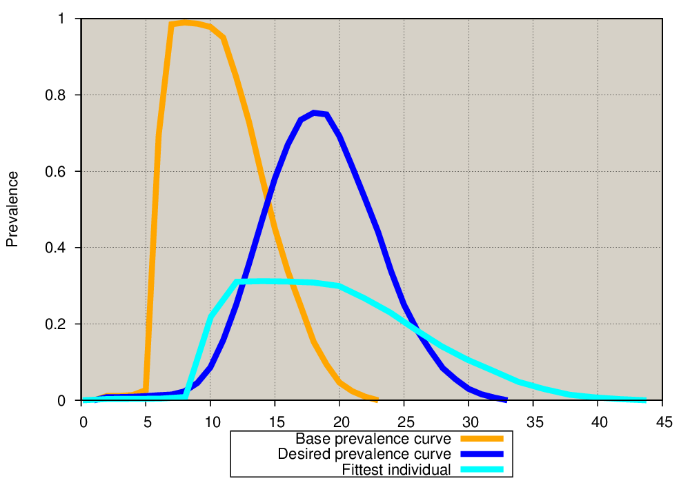
Each of those 2000 scenarios output a prevalence curve. A simple genetic algorithm (GA) programmed using DEAP was used to find values of shift, lengthen, flatten that would transform the base prevalence curve (no vaccination) into the prevalence curve output from the scenario.

The example below shows the base prevalence curve (orange) and the prevalence curve output from the scenario (dark blue). In this specific example, vaccination occurred 170 days before infection, and the percent of individuals expected to become vaccine immune was 43%. The “initial guesses” for shift, lengthen, flatten are shown in grey. Through successive generations of crossover and mutation, the GA refines the initial guesses to find values that produce a good fit (light blue curve) as measured by RMSE.

Examining the fitted curves with the worst RMSE revealed that some curves fit poorly. An alternate way of calculating error was tested to attempt to improve the fit.

• Initial error calculation: Given a point on the desired prevalence curve, project a line straight up or down to the GA curve. The error is the difference in y-coordinates. This calculation may be especially sensitive to cases where there are steep inclines or declines in the curve.
• Second error calculation: Given a point on the desired prevalence curve, find the shortest straight-line distance from that point to a point on the GA curve. The error is that shortest distance.

The second error calculation improved the fit when tried on some of the cases that initially had poor fits.

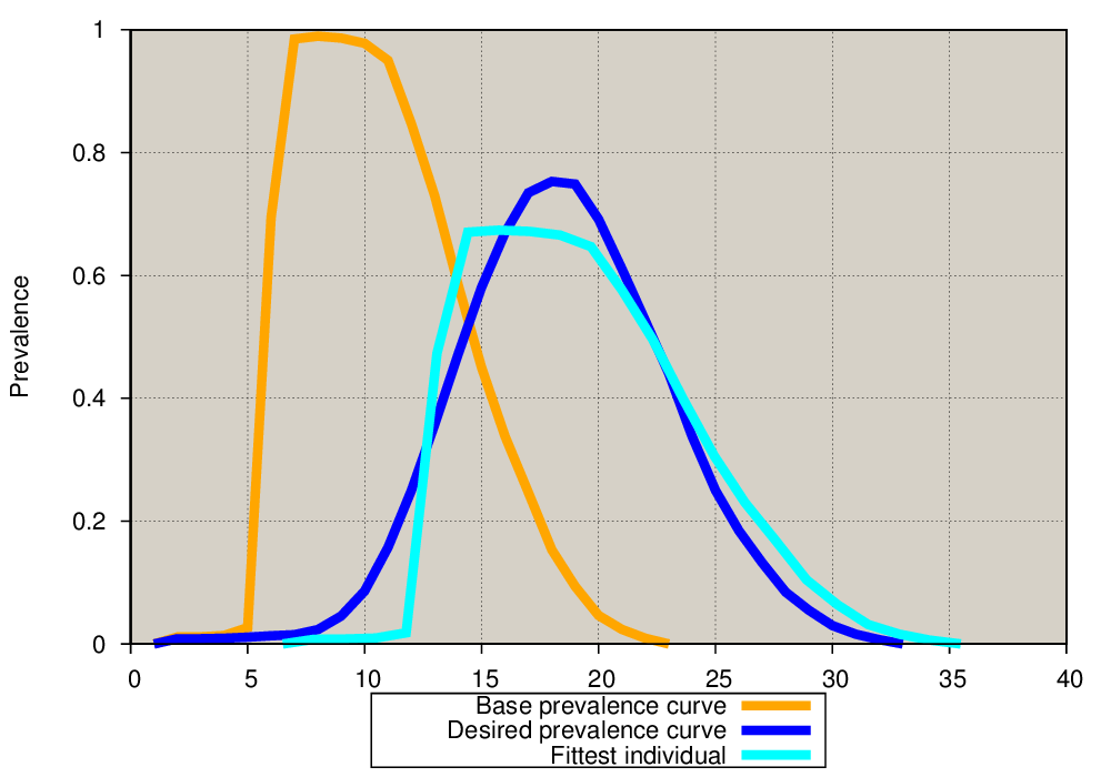Initial error calculation	Second error calculation

Even with the better error calculation, there are still a small number of cases with poor fits. When infection occurs just as vaccine immunity is running out, a bimodal prevalence curve can be produced. No values for shift, lengthen, flatten of a unimodal base prevalence curve will produce a good fit for these cases.

The fitted curves were turned into a regression problem, in which 3 outputs must be predicted given 28 inputs. The 3 outputs are the values for shift, lengthen, flatten. The 28 inputs were derived from the existing herd-level parameters that are readily available in ADSM, plus the two new parameters, percent of individuals expected to become vaccine immune and timing of vaccination relative to infection.

##Experiment 3 results

The regression models for the vaccination-then-infection runs were:

• shift = e^(2.3925 - .7178×i28 + .9181×i28²) – 10
• lengthen = e^(-.1547 + 1.2276×i28 – 1.4369×i28²)
• flatten = .8830 - .0012×i27 - 1.0969×i28 + .2359×i28²

The regression models for the infection-then-vaccination runs were:

• shift = 0
• lengthen = 1.0588 - .0100×i27 + .0002×i27² + .0485×i28
• flatten = 1.0126 - .1894×i2 + .0292×i27 - .0007*i27² + .1650×i28 - .2816×i28²

Where

• i2 = 25% point in the herd-level latent period, that is, the point on the x-axis where 25% of the area under the probability density function lies to the left of that point
• i27 = day of vaccination relative to day of infection
• i28 = fraction of individuals expected to become vaccine immune (0–1.0)