Basics of Stochastic Modeling - NAVADMC/ADSM GitHub Wiki

Biological processes display inherent variability. Take the height of the human male, for example, which can range from about 150 cm to 210 cm, although the average is close to 177 cm in the United States. If you wanted to develop a computer model to predict the amount of cloth needed to make x number of pairs of pants and you needed to include human male height as a variable, you could do so in two ways.

The first method would incorporate height as a single value, i.e. 177 cm, and assume that all men are that height. This method is called deterministic modeling because the value of the variable height has already been determined. If you wanted to estimate the amount of fabric needed to make 1,000 pairs of pants with a deterministic model, you would run the model just once to calculate the amount of fabric needed for one pair, then multiply the results by 1,000. Running the model more than once is not necessary, because the input variable is fixed and the results would be the same each time.

The second method would be to incorporate height as a distribution of values representative of the natural range. If the model is run several times, and if a different value is drawn at random from this distribution for each run, the results will be slightly different each time. This method is called stochastic (being or having a random variable) modeling because height is not a fixed value but is drawn randomly from a distribution. Values with higher probability of occurring (i.e., heights close to 177 cm) are more likely to be drawn than values at the extreme ends or “tails” of the distribution. In figure 3 1, we can see that values below 161cm are drawn 5 percent of the time, and values above 193 cm are drawn 5% of the time. Thus, 90 percent of the time, the value of height will be between 161cm and 193 cm.

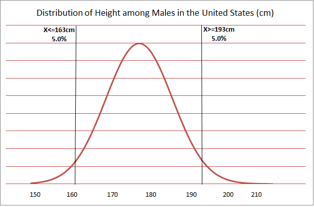
Figure 3-1

In a stochastic model, inputs and outputs are distributions. In our example, running a stochastic model just once is not particularly informative. However, by running the model for 1,000 iterations, we get 1,000 different estimates of how much fabric is needed for one pair of pants. These estimates form a distribution. To estimate the fabric needed for 1,000 pairs of pants, we simply sum the 1,000 estimates. Results of stochastic models incorporate variability, whereas results from deterministic models do not. We can improve our model by incorporating additional stochastic variables, such as the amount of fabric used per inch of height, which is affected by waist size and pant style.

ADSM is a stochastic model and incorporates variability using probabilities, distributions, and relationships. A distribution is used when the variability in a parameter is assumed to be random. The distribution describes the range of values a variable can take and how likely those values are to be selected. Model parameters described as distributions include the length of an infectious period and the distance that animals are likely to be transported. A relationship is used when the variability in one parameter is due to another factor. A relationship describes one variable as a function of another. Model parameters described as relationships include the probability of detecting an infectious herd—which is a function of time since the herd was infected— and the number of herds that can be depopulated per day— which is a function of time since the outbreak was detected.

Material Adapted from the User’s Guide for the North American Animal Disease Spread Model for NAADSM version 3.2.18