PICRUSt tutorial - LangilleLab/microbiome_helper GitHub Wiki
Introduction
This lab will walk you through the basic steps of using PICRUSt to make functional predictions (e.g. predicted metagenome) from your 16S data.
It uses an OTU table that has already been generated for use with PICRUSt. PICRUSt currently can only use an OTU table with GreenGene OTU identifiers which is the output from closed-reference picking or by filtering out de-novo OTUs after open-reference picking. Instructions for generating your OTU table for PICRUSt.
The data we will be using in this lab comes from the stool of three groups of mice that are of different ages (e.g. young, middle, and old).
You should attempt to answer tutorial questions on your own and then check the answer sheet to make sure you are on track.
If you are looking to use your own OTU table you might want to check out the PICRUSt Workflow.
Author: Morgan Langille
Contributions by: Gavin Douglas
First Created: June 2016
Last Edited: June 2017
Requirements
- Basic unix skills
- (This is a good introductory tutorial: http://korflab.ucdavis.edu/bootcamp.html)
- Microbiome Helper VirtualBox (install it and ensure it is working)
- Tutorial Data
Initial Setup
Open a terminal window by clicking on the little black box icon
Now we need to download the data using 'wget':
wget https://www.dropbox.com/s/v51fiyw5brauu2n/picrust_data.zip?dl=1 -O picrust_data.zip
Now decompress the data using "unzip" command and change into that directory:
unzip picrust_data.zip
cd picrust_data
Running PICRUSt
In your working directory you should have an OTU table called "otus.biom" and a mapping file "map.tsv". The OTU table has been produced within QIIME using the GreenGenes reference database. The mapping file is just a tab-delimited text file that has sample ids in the first column and a couple of additional columns with metadata for each sample. Take a look at these files:
less map.tsv
biom head -i otus.biom
biom summarize-table -i otus.biom
- Q1) How many samples are there in the dataset?
- Q2) What kind of metadata do we have about each of the samples?
The first step is to correct the OTU table based on the predicted 16S copy number for each organism in the OTU table:
normalize_by_copy_number.py -i otus.biom -o otus_corrected.biom
Note that this is just a normal OTU table which then could be used for other analyses.
If you want to look at the before and after correction you can use the biom tools to convert it to plain text:
biom convert -i otus_corrected.biom -o otus_corrected.txt --to-tsv --header-key taxonomy
biom convert -i otus.biom -o otus.txt --to-tsv --header-key taxonomy
Now you can look at them using less:
less otus.txt
# Constructed from biom file
#OTU ID	9Y-June1	10Y-June1	8Y-May23	10Y-May23	6Y-June1	9Y-May23	Y7-Aug14	Y7-Aug15	6Y-May23	M11-Aug14	M11-Aug15	M11-Jul13	11M-May23	M13-Jul13	13M-May23	2E-Aug14	2E-Aug15	2E-May24	4E-June1	1E-Aug16	1E-May23	taxonomy
181348	1.0	0.0	0.0	0.0	0.0	1.0	0.0	0.0	1.0	0.0	0.0	0.0	0.0	0.0	0.0	6.0	15.0	3.0	4.0	7.0	0.0	k__Bacteria;  p__Firmicutes;  c__Clostridia;  o__Clostridiales;  f__Lachnospiraceae;  g__Coprococcus;  s__
318732	0.0	0.0	1.0	0.0	0.0	0.0	0.0	0.0	2.0	5.0	9.0	7.0	1.0	5.0	3.0	0.0	2.0	0.0	0.0	0.0	0.0	k__Bacteria;  p__Firmicutes;  c__Clostridia;  o__Clostridiales;  f__;  g__;  s__
244484	0.0	0.0	0.0	2.0	0.0	1.0	0.0	1.0	4.0	0.0	2.0	0.0	2.0	1.0	0.0	0.0	1.0	0.0	2.0	0.0	1.0	k__Bacteria;  p__Firmicutes;  c__Clostridia;  o__Clostridiales;  f__Ruminococcaceae;  g__;  s__
(etc.)
less otus_corrected.txt
#OTU ID	9Y-June1	10Y-June1	8Y-May23	10Y-May23	6Y-June1	9Y-May23	Y7-Aug14	Y7-Aug15	6Y-May23	M11-Aug14	M11-Aug15	M11-Jul13	11M-May23	M13-Jul13	13M-May23	2E-Aug14	2E-Aug15	2E-May24	4E-June1	1E-Aug16	1E-May23	taxonomy
181348	0.333333333333	0.0	0.0	0.0	0.0	0.333333333333	0.0	0.0	0.333333333333	0.0	0.0	0.0	0.0	0.0	0.0	2.0	5.0	1.0	1.33333333333	2.33333333333	0.0	k__Bacteria;  p__Firmicutes;  c__Clostridia;  o__Clostridiales;  f__Lachnospiraceae;  g__Coprococcus;  s__
318732	0.0	0.0	0.333333333333	0.0	0.0	0.0	0.0	0.0	0.666666666667	1.66666666667	3.0	2.33333333333	0.333333333333	1.66666666667	1.0	0.0	0.666666666667	0.0	0.0	0.0	0.0	k__Bacteria;  p__Firmicutes;  c__Clostridia;  o__Clostridiales;  f__;  g__;  s__
244484	0.0	0.0	0.0	1.0	0.0	0.5	0.0	0.5	2.0	0.0	1.0	0.0	1.0	0.5	0.0	0.0	0.5	0.0	1.0	0.0	0.5	k__Bacteria;  p__Firmicutes;  c__Clostridia;  o__Clostridiales;  f__Ruminococcaceae;  g__;  s__
(etc.)
As you can see the otus_corrected.txt file has "normalized" the OTU table according to the PICRUSt 16S copy number predictions. By looking at the differences between the two OTU files you can tell what the predicted 16S copy number is for each OTU.
- Q3) What is the predicted 16S copy number for OTU 181348?
- Q4) What is the predicted 16S copy number for OTU 244484?
Ok, now lets actually make our functional predictions of KEGG Ortholog (KOs) predictions using the corrected OTU table as input:
predict_metagenomes.py -i otus_corrected.biom -o ko_predictions.biom
We can check out these KO predictions again by converting the BIOM file first:
biom convert -i ko_predictions.biom -o ko_predictions.txt --to-tsv --header-key KEGG_Description
# Constructed from biom file
#OTU ID	9Y-June1	10Y-June1	8Y-May23	10Y-May23	6Y-June1	9Y-May23	Y7-Aug14	Y7-Aug15	6Y-May23	M11-Aug14	M11-Aug15	M11-Jul13	11M-May23	M13-Jul13	13M-May23	2E-Aug14	2E-Aug15	2E-May24	4E-June1	1E-Aug16	1E-May23	KEGG_Description
K01365	0.0	0.0	0.0	0.0	0.0	0.0	0.0	0.0	0.0	0.0	0.0	0.0	0.0	0.0	0.0	0.0	0.0	0.0	0.0	0.0	0.0	cathepsin L [EC:3.4.22.15]
K01364	0.0	0.0	0.0	0.0	0.0	0.0	0.0	0.0	0.0	0.0	0.0	0.0	0.0	0.0	0.0	0.0	0.0	0.0	0.0	0.0	0.0	streptopain [EC:3.4.22.10]
K01361	18.0	20.0	9.0	4.0	11.0	4.0	9.0	6.0	6.0	7.0	10.0	11.0	9.0	11.0	8.0	32.0	8.0	15.0	17.0	8.0	9.0	lactocepin [EC:3.4.21.96]
K01360	0.0	0.0	0.0	0.0	0.0	0.0	0.0	0.0	0.0	0.0	0.0	0.0	0.0	0.0	0.0	0.0	0.0	0.0	0.0	0.0	0.0	proprotein convertase subtilisin/kexin type 2 [EC:3.4.21.94]
K01362	3587.0	3559.0	3868.0	3428.0	3872.0	3462.0	3432.0	1913.0	2436.0	3219.0	3248.0	3081.0	3372.0	2602.0	3494.0	3566.0	3527.0	2616.0	3133.0	3457.0	2212.0	None
K02249	0.0	0.0	0.0	0.0	0.0	0.0	0.0	0.0	0.0	0.0	0.0	0.0	0.0	0.0	0.0	0.0	0.0	0.0	0.0	0.0	0.0	competence protein ComGG
K05841	0.0	0.0	0.0	0.0	0.0	0.0	0.0	0.0	0.0	0.0	0.0	0.0	0.0	0.0	0.0	0.0	0.0	0.0	0.0	0.0	0.0	sterol 3beta-glucosyltransferase [EC:2.4.1.173]
Note: Default predictions from PICRUSt are KOs (KEGG Orthologs) but PICRUSt can also predict COGs and Rfams.
PICRUSt can also collapse KOs to KEGG Pathways. Note that one KO can map to many KEGG Pathways so a simple mapping wouldn't work here. Instead, we use the PICRUSt script "categorize_by_function.py":
categorize_by_function.py -i ko_predictions.biom -c KEGG_Pathways -l 3 -o pathway_predictions.biom
Again lets look at the output:
biom convert -i pathway_predictions.biom -o pathway_predictions.txt --to-tsv --header-key KEGG_Pathways
# Constructed from biom file
#OTU ID	9Y-June1	10Y-June1	8Y-May23	10Y-May23	6Y-June1	9Y-May23	Y7-Aug14	Y7-Aug15	6Y-May23	M11-Aug14	M11-Aug15	M11-Jul13	11M-May23	M13-Jul13	13M-May23	2E-Aug14	2E-Aug15	2E-May24	4E-June1	1E-Aug16	1E-May23	KEGG_Pathways
1,1,1-Trichloro-2,2-bis(4-chlorophenyl)ethane (DDT) degradation	11.0	21.0	10.0	7.0	14.0	4.0	8.0	1.0	4.0	0.0	0.0	0.0	1.0	0.0	0.0	1.0	1.0	2.0	4.0	2.0	1.0	Metabolism; Xenobiotics Biodegradation and Metabolism; 1,1,1-Trichloro-2,2-bis(4-chlorophenyl)ethane (DDT) degradation
ABC transporters	200982.0	174898.0	195247.0	255298.0	147766.0	254328.0	306731.0	490225.0	363852.0	217743.0	231867.0	239470.0	201328.0	237358.0	189880.0	199125.0	342119.0	294970.0	213939.0	229000.0	451627.0	Environmental Information Processing; Membrane Transport; ABC transporters
Adherens junction	0.0	0.0	0.0	0.0	0.0	0.0	0.0	0.0	0.0	0.0	0.0	0.0	0.0	0.0	0.0	0.0	0.0	0.0	0.0	0.0	0.0	Cellular Processes; Cell Communication; Adherens junction
Adipocytokine signaling pathway	6486.0	6300.0	7408.0	6562.0	7205.0	6982.0	6139.0	4365.0	5299.0	7160.0	7528.0	6977.0	8475.0	6064.0	7827.0	7404.0	7462.0	6411.0	7082.0	7654.0	5580.0	Organismal Systems; Endocrine System; Adipocytokine signaling pathway
African trypanosomiasis	28.0	25.0	40.0	42.0	23.0	26.0	188.0	33.0	22.0	62.0	63.0	43.0	19.0	12.0	29.0	19.0	24.0	12.0	9.0	22.0	9.0	Human Diseases; Infectious Diseases; African trypanosomiasis
Alanine, aspartate and glutamate metabolism	94807.0	90632.0	103163.0	103640.0	96543.0	104717.0	106172.0	112557.0	105979.0	93152.0	100320.0	98573.0	101380.0	90366.0	98759.0	100108.0	113079.0	103468.0	98339.0	104441.0	115040.0	Metabolism; Amino Acid Metabolism; Alanine, aspartate and glutamate metabolism
PICRUSt can directly connect the OTUs that are contributing to each KO by using the ''metagenome_contributions.py'' script. Here we specify 6 different KO ids. Usually the choice of KO ids would be driven by KOs that you are interested in, or KOs that are statistically signficant across your sample groupings.
metagenome_contributions.py -i otus_corrected.biom -l K01727,K01194,K01216,K11049,K00389,K00449 -o metagenome_contributions.txt
This is just a regular text file so can browse without conversion:
less metagenome_contributions.txt
The output should look like this:
Gene    Sample  OTU     GeneCountPerGenome      OTUAbundanceInSample    CountContributedByOTU   ContributionPercentOfSample     ContributionPercentOfAllSamples Kingdom Phylum  Class   Order   Family  Genus   Species
K01727  9Y-June1        190026  1.0     1.66666666667   1.66666666667   0.251889168766  0.000792700810933       k__Bacteria      p__Bacteroidetes        c__Bacteroidia  o__Bacteroidales        f__Rikenellaceae       g__AF12  s__
K01727  9Y-June1        4331760 3.0     1.0     3.0     0.453400503778  0.00142686145968        k__Bacteria      p__Bacteroidetes        c__Bacteroidia  o__Bacteroidales        f__Rikenellaceae       g__      s__
K01727  9Y-June1        2594570 1.0     0.333333333333  0.333333333333  0.0503778337531 0.000158540162187       k__Bacteria      p__Bacteroidetes        c__Bacteroidia  o__Bacteroidales        f__Rikenellaceae       g__      s__
K01727  9Y-June1        1106050 1.0     0.333333333333  0.333333333333  0.0503778337531 0.000158540162187       k__Bacteria      p__Bacteroidetes        c__Bacteroidia  o__Bacteroidales        f__Rikenellaceae       g__PW3   s__
K01727  9Y-June1        3090117 1.0     0.2     0.2     0.0302267002519 9.5124097312e-05        k__Bacteria      p__Bacteroidetes        c__Bacteroidia  o__Bacteroidales        f__[Barnesiellaceae]   g__      s__
K01727  9Y-June1        1051299 1.0     0.75    0.75    0.113350125945  0.00035671536492        k__Bacteria      p__Firmicutes   c__Bacilli      o__Lactobacillales      f__Streptococcaceae    g__Streptococcus         s__
K01727  9Y-June1        2617854 1.0     0.333333333333  0.333333333333  0.0503778337531 0.000158540162187       k__Bacteria      p__Bacteroidetes        c__Bacteroidia  o__Bacteroidales        f__Rikenellaceae       g__      s__
K01727  10Y-June1       190026  1.0     2.33333333333   2.33333333333   0.228758169935  0.00110978113531        k__Bacteria      p__Bacteroidetes        c__Bacteroidia  o__Bacteroidales        f__Rikenellaceae       g__AF12  s__
K01727  10Y-June1       4331760 3.0     0.666666666667  2.0     0.196078431373  0.00095124097312        k__Bacteria      p__Bacteroidetes        c__Bacteroidia  o__Bacteroidales        f__Rikenellaceae       g__      s__
K01727  10Y-June1       183395  1.0     0.2     0.2     0.0196078431373 9.5124097312e-05        k__Bacteria      p__Bacteroidetes        c__Bacteroidia  o__Bacteroidales        f__[Barnesiellaceae]   g__      s__
Each line in this file relates how much a single OTU (third column) contributes to a single KO (first column) within a single sample (second column). The fifth column contains the actual relative abundance contributed by this OTU, and the other columns contain other information about the abundance of the OTU and the percentage contribution of this OTU. The last columns provide the taxonomy information for the OTU.
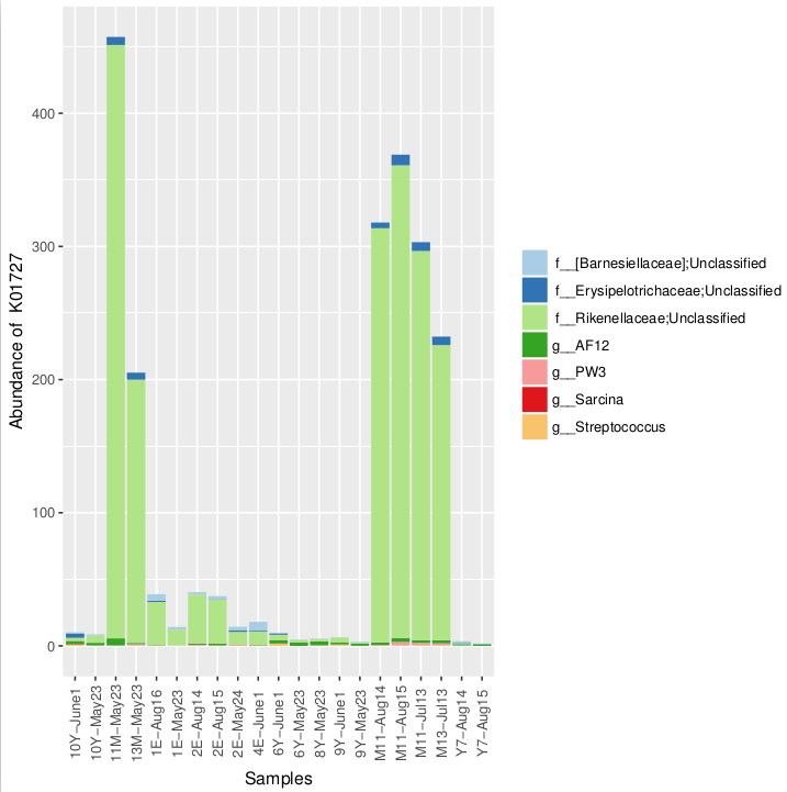
You could use your favourite plotting program (e.g. excel, sigmaplot, etc) to plot the information from columns 1-3 and column 5. We also provide an Rscript with Microbiome Helper that can be used to create stack bar charts of which taxa are contributing to functional abundances, which is shown below.
We can now create a stacked bar chart for K01727 with the below command.
/usr/local/prg/microbiome_helper/plot_metagenome_contributions.R --input metagenome_contributions.txt --output K01727_contrib.pdf --function_id K01727 --rank Genus
You should see the below plot. Note that there are a number of options that allow you to customize these figures. images/picrust_stacked_barchart.png
PICRUSt visualization and statistics in STAMP
STAMP takes two main files as input:
- the profile data which is a table that contains the abundance of features (i.e. taxonomic or functions)
- a group metadata file which provides more information about each of the samples in the profile data file.
The metadata file in our dataset is the map.tsv file, while the profile file can be generated using Microbiome Helper scripts.
Microbiome Helper provides several scripts for converting BIOM files into STAMP including those from PICRUSt.
First, we can use STAMP with the corrected OTU table by first converting it using the Microbiome Helper script:
biom_to_stamp.py -m taxonomy otus_corrected.biom > otus_corrected.spf
Alternatively, we can convert the BIOM file containing the PICRUSt KO predictions into a STAMP profile file:
biom_to_stamp.py -m KEGG_Description ko_predictions.biom > ko_predictions.spf
Lastly, we can do the same with the Pathway predictions:
biom_to_stamp.py -m KEGG_Pathways pathway_predictions.biom > pathway_predictions.spf
Lets load the pathway data in STAMP first. Start STAMP from within the Microbiome Helper Virtualbox image by clicking on the rainbow coloured flower on the left of the desktop.
Now load the pathway_predictions.spf file and the map.tsv file within STAMP (File->Load data).

Change Profile Level to "Level 3" which actually represents the KEGG Pathways. Then change the "Group Field" (top right) to "Age_Group".
Apply a multiple test correction (Benjamini-Hochberg FDR) and then view the individual KEGG Pathways using a "Box Plot" (instead of PCA plot) by changing the dropdown box in the lower left. This will open a new window the names of different pathways along with the Eta-squared, p-value, and corrected p-value. By clicking on each pathway a box plot will be drawn. You can order the pathways (for example by the corrected p-value), and you can also limit the list to only those that are statistically significant by checking the "Show only active features" box.
Q5) What is the most significant KEGG Pathway?
You should have a plot like the following.

If you like you can explore other visualizations with STAMP or attempt to load KOs instead within STAMP. For example, you should be able to answer the following question.
Q6) What is the most significant KO between Healthy and Sick using a multiple test corrected Welch's t-test?
Q7) Generate a bar plot for this KO.