PICRUSt Tutorial with de novo Variants - LangilleLab/microbiome_helper GitHub Wiki
Note this workflow was used as a placeholder while PICRUSt2 was being developed. Users interested in using de novo variants for metagenome prediction should check out the PICRUSt2 repository.
One drawback of using PICRUSt is that it restricts users to picking against OTUs in the Greengenes database. This is not ideal for several reasons including that a large proportion of OTUs are typically de novo and OTU picking is gradually being replaced by error correction approaches like DADA2 and deblur.
To get around this drawback the user can run the genome prediction steps of PICRUSt themselves (rather than having a pre-calculated supplied for reference OTUs). The below workflow will show users how they can run these steps themselves on DADA2 variants. The dataset we will be using is the output of our DADA2 16S tutorial. A description of this data and the accompanying metadata is available at the beginning of that tutorial. This approach is currently being refined so this will likely change over time. This tutorial is based partially on the steps laid out here: https://github.com/vmaffei/dada2_to_picrust.
Acquire data
If you are running this tutorial as part of EMBL-EBI's Metagenomics workshop then the tutorial files should already be on your computer. You can copy the zipped folder to the Desktop, unzip it, and enter the folder to get started.
cd ~/Desktop
cp ~/Documents/picrust_tutorial_Oct2017.zip ~/Desktop
unzip picrust_tutorial_Oct2017.zip
cd picrust_tutorial_Oct2017
Otherwise you can download the tutorial files by replacing the cp command above with the below wget command.
wget http://kronos.pharmacology.dal.ca/public_files/tutorial_datasets/picrust_tutorial_Oct2017.zip
Overview of data
In the picrust_tutorial_Oct2017 directory you will see output files from the DADA2 pipeline (the files produced by our DADA2 16S tutorial) and required files that will be used for the genome prediction steps.
dada2_out/contains the counts of the variants identified with DADA2 (seqtab_tax_rarified.biom) and their sequences in FASTA format (seqtab.fasta).map.txtcontains the metadata for each sample and will be used at the data analysis stage.img_gg_starting_files/contains IMG KEGG ortholog counts that were used to create PICRUSt's precalculated files for the Greengenes database. The counts of 16S rRNA copies is also found in this folder. This trait is important to keep track to normalize PICRUSt results. There are additional files which in this directory which will be described when needed.
Activate anaconda environment
Before proceeding with this workflow you will need to activate the qiime1 anaconda environment.
source ~/anaconda2/bin/activate qiime1
Create New Reference Tree
Trait predictions with PICRUSt are based on ancestral state reconstruction (ASR). This method requires a phylogenetic tree of all the taxa of interest (the study and reference sequences in this case). To make this tree we need to align all of these sequences of interest together.
The first step is to concatenate the study and reference 16S rRNA gene sequences into a single file. Note that the first argument below is the output of the DADA2 pipeline for our dataset. The second argument is the reference full-length 16S sequences for the subset of Greengenes OTUs that correspond to genomes in IMG with KEGG ortholog count data.
cat dada2_out/seqtab.fasta img_gg_starting_files/gg_13_5_img_subset.fasta > study_seqs_gg_13_5_img_subset.fasta
Next we need to align all of these sequences together. The below command will do this using PyNAST, which uses the full Greengenes reference alignment as a template.
align_seqs.py -e 90 -p 0.1 -i study_seqs_gg_13_5_img_subset.fasta -o study_seqs_gg_13_5_img_subset_pynast
Non-default options:
-e 90: Min sequence length of 90 to include in alignment.-p 0.1: Min percent identity of 10% to include in the alignment.
Filter low quality columns from alignment. This is important since the alignment is being made between full 16S sequences and shorter variants of variable regions.
filter_alignment.py -i study_seqs_gg_13_5_img_subset_pynast/study_seqs_gg_13_5_img_subset_aligned.fasta -o study_seqs_gg_13_5_img_subset_pynast
We can now run fasttree to build a phylogenetic tree based on this alignment. The below command is the multi-threaded version of fasttree (you need to export a shell variable specifying the number of threads).
export OMP_NUM_THREADS=9
FastTreeMP  -nt -gamma -fastest -no2nd -spr 4 -constraints img_gg_starting_files/99_otus_IMG_pruned_no_names_constraint.txt < study_seqs_gg_13_5_img_subset_pynast/study_seqs_gg_13_5_img_subset_aligned_pfiltered.fasta > study_seqs_gg_13_5_img_subset.tre
There is a lot going on in this command, so here is the breakdown:
-nt: specifies the alignment is of nucleotides.-gamma: rescale branch lengths and compute Gamma20-based likelihood.-fastest: speed up neighbour-joining phase.-no2nd: when used with-fastestyields an intermediate level of speed and search intensiveness.-spr 4: specifies 4 subtree-pruning-regrafting steps (see paper).-constraints img_gg_starting_files/99_otus_IMG_pruned_no_names_constraint.txt: file containing topology constraints for Greengenes sequences included in the tree (calculated in advance and based on the original Greengenes tree).< FILE: this specifies the input file.> FILE: this specifies the output file.
PICRUSt genome prediction
Start by formatting input tree and trait table. The below commands perform a few different checks of the input files and prepares them for the ASR step.
format_tree_and_trait_table.py -t study_seqs_gg_13_5_img_subset.tre -i img_gg_starting_files/gg_13_5_img_16S_counts.txt -o format/16S

format_tree_and_trait_table.py -t study_seqs_gg_13_5_img_subset.tre -i img_gg_starting_files/img_400_ko.tab -o format/KO -m img_gg_starting_files/gg_13_5_img_fixed.txt
Run ancestral state reconstruction steps for 16S rRNA gene counts to get estimates for every internal node in the tree. The default method is phylogenetic independent contrasts although there are other methods available as well.
ancestral_state_reconstruction.py -i format/16S/trait_table.tab -t format/16S/pruned_tree.newick -o asr/16S_asr_counts.tab -c asr/asr_ci_16S.tab
Now that we have the trait predictions for all internal nodes we can extend these 16S counts predictions to the tips of the tree (i.e. our study sequences of interest). Note that the ASR files for the KEGG orthologs have been pre-calculated.
predict_traits.py -i format/16S/trait_table.tab -t format/16S/reference_tree.newick -r asr/16S_asr_counts.tab -o predicted/16S_precalculated.tab -a -c asr/asr_ci_16S.tab
You could also run this command to run ASR for the KO table. These commands can take > 30 minutes so we have made the output files of predict_traits.py available in img_gg_starting_files/precalc_predict if you want to skip these commands.
ancestral_state_reconstruction.py -i format/KO/trait_table.tab -t format/KO/pruned_tree.newick -o asr/KO_asr_counts.tab -c asr/asr_ci_KO.tab

predict_traits.py -i format/KO/trait_table.tab -t format/KO/reference_tree.newick -r asr/KO_asr_counts.tab -o predicted/KO_precalculated.tab -a -c asr/asr_ci_KO.tab
The output of these commands is the table of trait counts across study and reference variants for both 16S copy number and KOs. **Since there is variability in the alignment step it is likely your output will differ at least slightly from the results shown below. You can use our pre-calculated predictions if you want to re-generate the below plots, which are in img_gg_starting_files/precalc_predict. If you want to use the previously generated predicted tables for the below commands then you should first run this command to overwrite the tables in predicted/: cp img_gg_starting_files/precalc_predict/* predicted/.
Add metadata to KO table
You will need to add the metadata to the KEGG prediction table before proceeding. For this dataset this can easily be done with the below commands (the echo command is just adding a newline to the end of the trait table).
echo "" >> predicted/KO_precalculated.tab
cat img_gg_starting_files/metadata/precalc_meta >> predicted/KO_precalculated.tab
Get predictions per sample based on the abundance of each variant.
Now that we have the predicted trait abundances per variant (i.e. for their predicted genome) we can get the predicted trait abundances for each sample (i.e. the predicted metagenome). The first step in this process is to normalize the variant abundances by the predicted 16S copy number. This is important so that the abundances of gene families and other functions are comparable in downstream steps.
Note that the precalculated trait tables that we generated above are specified with the -c option in the below commands.
normalize_by_copy_number.py -i dada2_out/seqtab_tax_rarified.biom -c predicted/16S_precalculated.tab -o seqtab_tax_rarified_norm.biom
Now that the variant table is normalized by 16S copy number we can determine the predicted number functions in each sample. Essentially this command multiplies each variant's normalized abundance by the abundance of each function in the precalculated table.
predict_metagenomes.py -i seqtab_tax_rarified_norm.biom -c predicted/KO_precalculated.tab -o seqtab_tax_rarified_norm_ko.biom
The above command generated predicted metagenomes for KEGG orthologs (i.e. the gene families). However, often we are interested in more readily interpretable categories like pathways. To collapse the KEGG orthologs to KEGG pathways the below command can be used.
categorize_by_function.py -i seqtab_tax_rarified_norm_ko.biom -o seqtab_tax_rarified_norm_ko_l3.biom -c KEGG_Pathways -l 3
Breakdown of Taxonomic Contributions
Although predicted metagenomes are useful often users want to know which taxa are actually conferring specific functions. To this end the below command will output a textfile that states what abundance of a function is being conferred by a given variant (and their taxonomic assignment). The below command will output these predicted contributions for two KEGG orthologs: K08602 and K03699.
metagenome_contributions.py -i seqtab_tax_rarified_norm.biom -l K08602,K03699 -o metagenome_contributions.txt -c predicted/KO_precalculated.tab
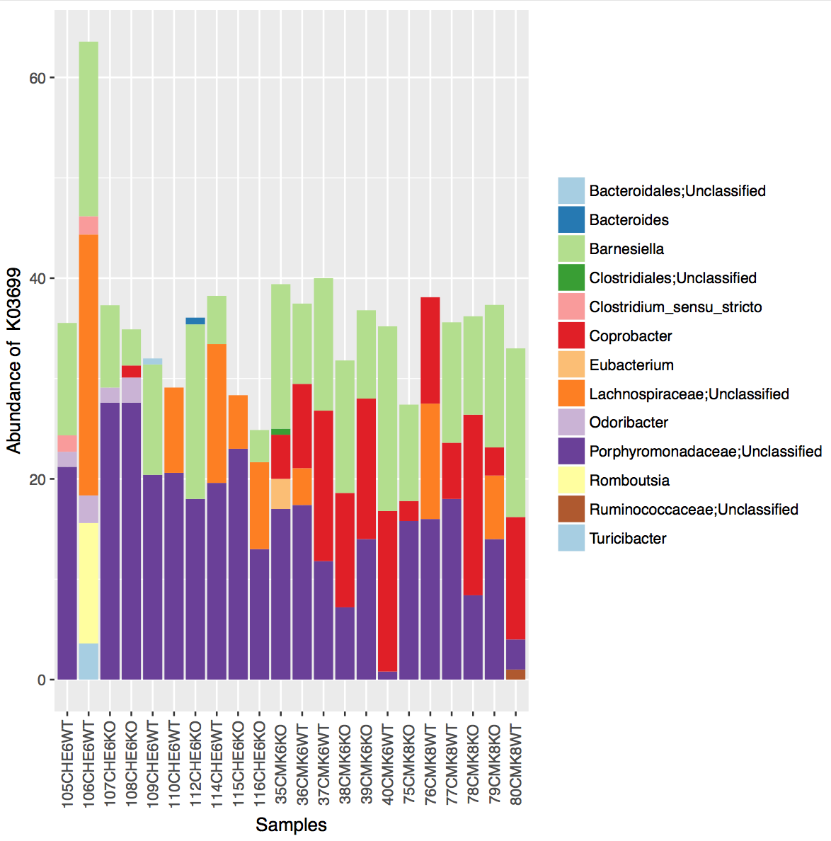
To visualize these contributions you can plot stacked barcharts of abundances conferred at a specified taxonomic labels (Genus below).
plot_metagenome_contributions.R --input metagenome_contributions.txt --output K03699_contrib.pdf --function_id K03699 --rank Genus
Your plot will look like this:
images/dada2_16S_tutorial/picrust_contrib_stacked_barchart_new.png
Testing for Statistical Differences with STAMP
There are numerous approaches that could be used to test for statistical differences in predicted function abundances between sample groupings. One simple approach is to use STAMP (as described in our 16S DADA2 tutorial).
The predicted metagenome tables can be converted to STAMP format with these commands.
biom_to_stamp.py -m "KEGG_Description" seqtab_tax_rarified_norm_ko.biom > seqtab_tax_rarified_norm_ko.spf
biom_to_stamp.py -m "KEGG_Pathways" seqtab_tax_rarified_norm_ko_l3.biom > seqtab_tax_rarified_norm_ko_l3.spf
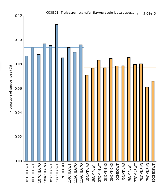
These .spf files can be read into STAMP with the metadata file (map.txt) and analyses can be run using the same approach as for taxonomic features. Change the Group field to "Source" and to a Two groups test. Select the two-sided Welch's t-test. Change plot-type to barplot and sort KOs by their raw P-values. You should see a barplot of top KO like this:
images/dada2_16S_tutorial/ex_ko_barplot.png
You can also run similar tests on the KEGG pathways. You can read in the SPF for this data as well with the same settings as above except set the Profile level to Level_3. Boxplots are another useful way to visualize the data. A boxplot of the top KEGG pathway after multiple-test correction should look like this:
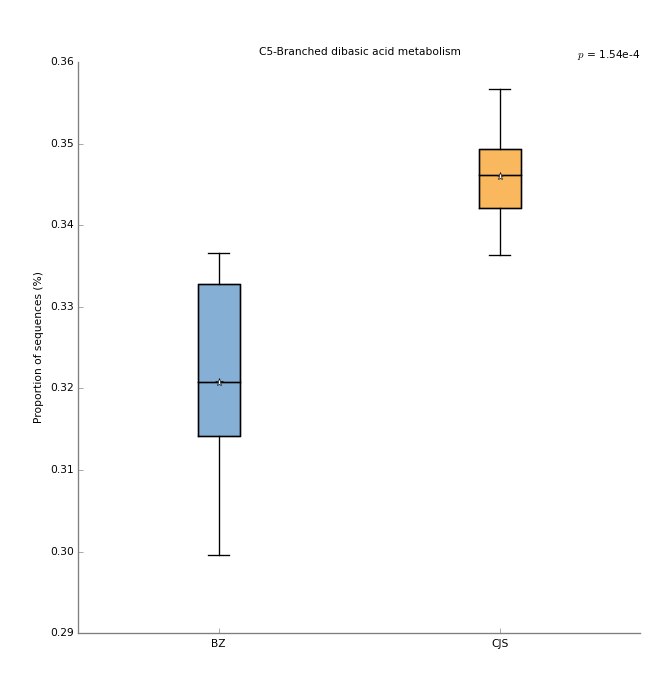