Metagenomics Tutorial (HUMAnN2) - LangilleLab/microbiome_helper GitHub Wiki

Introduction

This tutorial is set-up to walk you through the process of determining the taxonomic and functional composition of several metagenomic samples. It covers the use of Metaphlan2 (for taxonomic classification), HUMAnN2 (for functional classification), and STAMP (for visualization and statistical evaluation).

Throughout the tutorial, there are several questions to ensure that you are understanding the process (and not just copy and pasting). You can check the answer sheet after you have answered them yourself.

We'll be using a subsampled version of the metagenomics dataset from Schmidt et al. (PLoS ONE 2014) that investigated changes in the oral microbiome associated with oral cancers. Note: since these files have been drastically subsampled they do not represent typical metagenomics raw files. For instance, many more taxonomic and functional classifications would be output if the full datasets were used. However, due to the shallow read depth the running time of the workflow is extremely fast!

Authors: Morgan Langille and Gavin Douglas

First Created: June 2017

Last Updated: 5 Oct 2017

Requirements

Basic unix skills (there are many tutorials online such as this one)
Tutorial data (commands to download are below)
Full Microbiome Helper Virtual Box Image

Initial Setup

Download the tutorial data, save it to the Desktop (within Ubuntu), unzip the folder, and enter this folder. You can do this using the below commands.

Open a terminal/console and change to the directory containing the tutorial data:
(paste the below command with your mouse, you probably wont be able to copy/paste text in the VBox with keyboard commands)

cd ~/Desktop/  
wget http://kronos.pharmacology.dal.ca/public_files/MH/tutorial_datasets/mgs_tutorial_Oct2017.zip
unzip mgs_tutorial_Oct2017.zip   
cd mgs_tutorial_Oct2017

Explore Samples

The first step in any metagenomics pipeline should be to explore your raw files. For this tutorial there should be a "mapping file", which contains information about each of the samples called map.txt, along with the sequence data for each sample contained within separate FASTQ files within the directory raw_data.

Lets take a look at map.txt using less (type q to quit out of the program when done)

less map.txt

You will have noticed that this map file contains four columns with the first being sample ids, then sample type (Cancer or Normal), sex, and the individual. Samples nearby an oral tumor and distal from oral tumors were taken for each individual.

Remember you can count the lines of a file using wc -l. For example,

wc -l map.txt

Q1) How many samples are there in total (you can either look at the map.txt file or count the FASTQ files)?

Q2) How many samples are there of each sample type?

Before continuing let's take a look at the raw sequence files themselves. Typically it's better to keep these files in gzipped format to save disk space. However, since several commands below require the files to be uncompressed we can gunzip them now:

gunzip raw_data/*gz

FASTQ format is currently the most common format for raw sequencing reads. In this format, information for each read is split over 4 lines: a header (i.e. the read name and other details), the sequence, a line containing "+", and the quality scores for each nucleotide.

To visualize this we can look at the first 8 lines of one of the FASTQs using the head command:

head -n 8 raw_data/p136C_R1.fastq

@SRR3586062.883556
CTTGGGGCTGCTGAGCTTCATGCTCCCCTCCTGCCTCAAGGACAATAAGGAGATCTTCGACAAGCCTGCAGCAGCTCGCATCGACGCCCTCATCGCTGAGG
+
CCCFFFFFHHHHHIJJJJJJJIJIJJJJGIJDGIJEIIJIJJJJJJJJIJJJJIJJIJJJJJHHHFFFFECEEEDDDDD?BDDDDDDBDDDDDDDDBBBDD
@SRR3586062.3376311
GACGGTGTCCTCAGGACCCTTCAGTGCCTTCATGATCTGCTCAGAGGTGATGGAGTCACGGACGAGATTCGTCGTGTCAGCACGTAGGATGCGGTCGCCTG
+
@@@DDDDAFF?DF;EH+ACHIIICHDEHGIGBFE@GCGDGG?D?G@BGHG@FHCGC;CC:;8ABH>BECCBCB>;8ABCCC@A@#################

Q3) To save time each sample has been subsampled to a relatively low number of reads. How many sequences are there in each FASTQ?

For your own data you may identify outlier samples with low read depth at this stage. It would also be advisable to explore the quality of your data with a tool like FASTQC.

Pre-processing

Although you could run this workflow on all of the test files, we will just be running them on one sample, which is in the raw_data_example folder and should already be gunzipped.

Two major pre-processing steps need to be performed on shotgun metagenomics sequences: quality filtering of reads and screening out of contaminant reads.

Trimmomatic is one popular tool for filtering and trimming next-generation sequencing data. Typically you would first explore the quality of your data to choose sensible cut-offs using FASTQC or a similar alternative. Below we will run Trimmomatic on our test file with some typical cut-offs.

It is also important to screen out contaminant sequences. This is because the strength of shotgun metagenomics is also its weakness: all DNA in your samples will be sequenced with similar efficiencies. This is a problem when host microbiome samples are taken since it's possible to get substantial amounts of host DNA included in your raw sequences. You should screen out these contaminant sequences before running taxonomic and functional classification. It's also a good idea to screen out PhiX sequences in your data: this virus is a common sequencing control since it has such a small genome.

Below we will screen out reads that map to the human and/or PhiX genomes with Bowtie2 in paired-end mode. If your samples were taken from a different host you will need to map your reads to that genome instead. (We will just run one of our samples for now).

kneadData is a helpful wrapper of both Trimmomatic and Bowtie2. You can use the below command to run kneaddata on a single sample.

kneaddata -i raw_data_example/p144C_R1.fastq -i raw_data_example/p144C_R2.fastq -o kneaddata_out \
-db /home/shared/bowtiedb/GRCh38_PhiX --trimmomatic /usr/local/prg/Trimmomatic-0.36/ \
-t 4 --trimmomatic-options "SLIDINGWINDOW:4:20 MINLEN:50" \
--bowtie2-options "--very-sensitive --dovetail" --remove-intermediate-output

The options above are:

-i Input FASTQ file. This option is given twice for paired-end data.
-o Output directory.
-db Path to bowtie2 database.
--trimmomatic Path to Trimmomatic folder containing jarfile.
-t 4 Number of threads to use (4 in this case).
--trimmomatic-options Options for Trimmomatic to use, in quotations ("SLIDINGWINDOW:4:20 MINLEN:50" in this case). See Trimmomatic website for more options.
--bowtie2-options Options for bowtie2 to use, in quotations. The options "--very-sensitive" and "--dovetail" in this set alignment parameters to be very sensitive and sets cases where mates extend past each other to be concordant (i.e. they will be called as contaminants and be excluded).
--remove-intermediate-output Intermediate files, including large FASTQs, will be removed.

The output files are in kneaddata_out, which also contains a logfiles containing the commands run. There are a number of FASTQs in this directory, but we are only interested in the files ending in "_paired_1.fastq" and "_paired_2.fastq", which are the forward and reverse reads in pairs that both passed the filtering criteria and were not mapped as contaminants. If you are interested in seeing which reads were called as contaminants they are in the "contam" FASTQs. The passing reads where the other read-pair failed either pre-processing step are in the "unmatched" FASTQs. These sequences can still be useful, but in this case we will exclude them from downstream steps. Note that you should ignore the "R1" in the output files - the reverse reads will end with "_2.fastq".

To run kneaddata on all samples with a single command check out this page, which describes how this can be done using the parallel command.

You can get a summary of read counts passed at each step broken down by paired and unmatched reads with this command:

kneaddata_read_count_table --input kneaddata_out --output kneaddata_read_counts.txt

Q4) How many reverse reads for p144C passed the Trimmomatic step without the other read in the pair (i.e. as an orphan)?

Lastly, since we didn't stitch the paired-end reads together at the beginning of this workflow we will concatenate the FASTQs together now before running Metaphlan2 and HUMAnN2 since these programs do not use paired-end information. We'll need to move the contaminated sequences to a different folder first since we are not interested in them and we will only retain read pairs where both forward and reverse reads passed the pre-processing steps.

mkdir kneaddata_out/contam_seq

mv kneaddata_out/*_contam_*fastq kneaddata_out/contam_seq

concat_paired_end.pl -p 4 --no_R_match -o cat_reads kneaddata_out/*_paired_*.fastq

Taxonomic and Functional Profiling with MetaPhlAn2 and HUMAnN2 Respectively

MetaPhlAn2 is a standalone tool and can be run with the metaphlan2.py command. It is easier to run a custom analysis with this script directly. However, since HUMAnN2 runs this script anyway (with default options unless specified otherwise) we can use the output files produced by this pipeline instead, which is simpler!

To begin with make sure the program humann2 is in your PATH. This program is frequently updated so it's a good idea to check what version you're running.

Q5) What version of HUMAnN2 are you using? What version of MetaPhlAn2?

Running the HUMAnN2 Pipeline (which includes MetaPhlAn2)

Both humann2 and metaphlan2.py come with a large number of options which could be useful (take a look by running each program with the -h option). Since humann2 can take a while to run we'll just run one sample for this tutorial (key output files are in the precalculated folder already).

humann2 --threads 1 --input cat_reads/p144C.fastq  --output humann2_out/

You should see a log of what HUMAnN2 is doing printed to screen:

Running metaphlan2.py ........

Found g__Fusobacterium.s__Fusobacterium_nucleatum : 22.70% of mapped reads
Found g__Neisseria.s__Neisseria_unclassified : 18.81% of mapped reads
Found g__Fusobacterium.s__Fusobacterium_periodonticum : 10.78% of mapped reads
Found g__Prevotella.s__Prevotella_melaninogenica : 10.48% of mapped reads
Found g__Haemophilus.s__Haemophilus_parainfluenzae : 9.52% of mapped reads
Found g__Gemella.s__Gemella_unclassified : 5.48% of mapped reads
Found g__Veillonella.s__Veillonella_unclassified : 3.84% of mapped reads
Found g__Sphingomonas.s__Sphingomonas_melonis : 2.01% of mapped reads
Found g__Gemella.s__Gemella_haemolysans : 1.16% of mapped reads

Total species selected from prescreen: 9

The MetaPhlAn2 output file is the "*bugs_list.tsv" in the temp folder within the output folder. You can take a look at it with less.

Your should see something like this:

#SampleID       Metaphlan2_Analysis
k__Bacteria     100.0
k__Bacteria|p__Fusobacteria     48.69306
k__Bacteria|p__Proteobacteria   30.34017
k__Bacteria|p__Firmicutes       10.48718
k__Bacteria|p__Bacteroidetes    10.47959
k__Bacteria|p__Fusobacteria|c__Fusobacteriia    48.69306
k__Bacteria|p__Proteobacteria|c__Betaproteobacteria     18.80684
k__Bacteria|p__Bacteroidetes|c__Bacteroidia     10.47959
k__Bacteria|p__Proteobacteria|c__Gammaproteobacteria    9.51996
k__Bacteria|p__Firmicutes|c__Bacilli    6.64301
k__Bacteria|p__Firmicutes|c__Negativicutes      3.84417

You can see that the output contains two columns, with the first column being the taxonomy name and the second column representing the relative abundance of that taxa (out of 100 total).

This output file provides summaries at each taxonomic level (e.g. phylum, class, family, genus, species, and sometimes strain level). At each taxonomic level the relative abundances will sum to 100.

If reads can only be assigned to a certain taxonomic level (e.g. say the family level), then MetaPhlAn2 will put those unassigned reads into a lower level taxonomic rank with the name "unclassified" appended.

For example lets pull out all the reads assigned to the genus Gemella using the grep command:

grep g__Gemella humann2_out/p144C_humann2_temp/p144C_metaphlan_bugs_list.tsv

You should get output like this:

k__Bacteria|p__Firmicutes|c__Bacilli|o__Bacillales|f__Bacillales_noname|g__Gemella	7.02294
k__Bacteria|p__Firmicutes|c__Bacilli|o__Bacillales|f__Bacillales_noname|g__Gemella|s__Gemella_unclassified	3.73681
k__Bacteria|p__Firmicutes|c__Bacilli|o__Bacillales|f__Bacillales_noname|g__Gemella|s__Gemella_haemolysans	2.08571
k__Bacteria|p__Firmicutes|c__Bacilli|o__Bacillales|f__Bacillales_noname|g__Gemella|s__Gemella_sanguinis	1.20042
k__Bacteria|p__Firmicutes|c__Bacilli|o__Bacillales|f__Bacillales_noname|g__Gemella|s__Gemella_haemolysans|t__Gemella_haemolysans_unclassified	2.08571
k__Bacteria|p__Firmicutes|c__Bacilli|o__Bacillales|f__Bacillales_noname|g__Gemella|s__Gemella_sanguinis|t__GCF_000204335	1.20042

You can see that 7.02% of the metagenome is predicted from organisms in the genus Gemella. More precisely: 2.09% are assigned to the species Gemella haemolysans, 1.20% to the species Gemella sanguinis, and 3.74% are assigned to s__Gemella_unclassified (which means MetaPhlAn2 can't determine species-level assignment).

Q6) What is the relative abundance of organisms unclassified at the species level for the genus Neisseria? (Remember to use the grep command)

Running HUMAnN2 on all FASTQs with GNU Parallel

You don't need to do this for the tutorial, but the below command could be used to run HUMAnN2 on each FASTQ using default options with GNU parallel to loop over each file. You can see our tutorial for more details on this command, but briefly:

-j indicates the number of jobs to run.
--eta outputs the expected time to finish as individual jobs end.
The files being looped over follow :::.
Everything within the single-quotes (') is the actual command being run on every file. The options within the quotes are for the particular tool being run and NOT parallel.
{} specifies each individual filename being looped over.
{/.} specifies the individual filename being looped over with the extension and PATH removed.

It's a good idea to run parallel with the --dry-run option the first time you are running a set of files. This option will echo the commands that would have been run to screen without running them. This can be very helpful for troubleshooting parallel syntax errors! Again you do not need to run this command, it just shows you how you could run humann2 on all FASTQs in cat_reads (this is useful when you want to loop over many samples!).

parallel -j 1 'humann2 --threads 1 --input {} --output humann2_out/{/.}' ::: cat_reads/*fastq

Setting the option --memory-use maximum will speed up the program if you have enough available memory.

Merging Metaphlan2 Results

We've placed all of the MetaPhlAn2 output files in precalculated/metaphlan2_out. All of these files can be merged into one table with this command:

/usr/local/prg/metaphlan2/utils/merge_metaphlan_tables.py precalculated/metaphlan2_out/*tsv > metaphlan2_merged.tsv

Note that this script merge_metaphlan_tables.py takes one or more MetaPhlAn2 output files as input and combines them into a single output file.

The merged output file should look like this:

ID      p136C_metaphlan_bugs_list       p136N_metaphlan_bugs_list       p143C_metaphlan_bugs_list       p143N_metaphlan_bugs_list       p144C_metaphlan_bugs_list       p144N_metaphlan_bugs_list       p146C_metaphlan_bugs_list       p146N_metaphlan_bugs_list       p153C_metaphlan_bugs_list       p153N_metaphlan_bugs_list       p156C_metaphlan_bugs_list       p156N_metaphlan_bugs_list
#SampleID       Metaphlan2_Analysis     Metaphlan2_Analysis     Metaphlan2_Analysis     Metaphlan2_Analysis     Metaphlan2_Analysis     Metaphlan2_Analysis
     Metaphlan2_Analysis     Metaphlan2_Analysis     Metaphlan2_Analysis     Metaphlan2_Analysis     Metaphlan2_Analysis     Metaphlan2_Analysis
k__Bacteria     100.0   100.0   99.19073        100.0   100.0   100.0   100.0   100.0   100.0   100.0   100.0   100.0
k__Bacteria|p__Actinobacteria   0.0514  0.42566 0.0     32.47169        0.0     12.48777        6.76551 6.93423 0.0     28.91843        0.0     6.1563
k__Bacteria|p__Actinobacteria|c__Actinobacteria 0.0514  0.42566 0.0     32.47169        0.0     12.48777        6.76551 6.93423 0.0     28.91843        0.0
     6.1563
k__Bacteria|p__Actinobacteria|c__Actinobacteria|o__Actinomycetales      0.0     0.0     0.0     32.47169        0.0     12.48777        6.76551 6.93423 0.0
     28.91843        0.0     6.1563
k__Bacteria|p__Actinobacteria|c__Actinobacteria|o__Actinomycetales|f__Actinomycetaceae  0.0     0.0     0.0     0.64587 0.0     0.0     0.0     0.0     0.0
     0.05704 0.0     0.0
k__Bacteria|p__Actinobacteria|c__Actinobacteria|o__Actinomycetales|f__Actinomycetaceae|g__Actinomyces   0.0     0.0     0.0     0.64587 0.0     0.0     0.0
     0.0     0.0     0.05704 0.0     0.0
k__Bacteria|p__Actinobacteria|c__Actinobacteria|o__Actinomycetales|f__Actinomycetaceae|g__Actinomyces|s__Actinomyces_odontolyticus      0.0     0.0     0.0
     0.0     0.0     0.0     0.0     0.0     0.0     0.05704 0.0     0.0
k__Bacteria|p__Actinobacteria|c__Actinobacteria|o__Actinomycetales|f__Actinomycetaceae|g__Actinomyces|s__Actinomyces_odontolyticus|t__Actinomyces_odontolyticus_unclassified    0.0     0.0     0.0     0.0     0.0     0.0     0.0     0.0     0.0     0.05704 0.0     0.0
k__Bacteria|p__Actinobacteria|c__Actinobacteria|o__Actinomycetales|f__Actinomycetaceae|g__Actinomyces|s__Actinomyces_viscosus   0.0     0.0     0.0     0.64587 0.0     0.0     0.0     0.0     0.0     0.0     0.0     0.0
k__Bacteria|p__Actinobacteria|c__Actinobacteria|o__Actinomycetales|f__Actinomycetaceae|g__Actinomyces|s__Actinomyces_viscosus|t__GCF_000175315  0.0     0.0
     0.0     0.64587 0.0     0.0     0.0     0.0     0.0     0.0     0.0     0.0
k__Bacteria|p__Actinobacteria|c__Actinobacteria|o__Actinomycetales|f__Corynebacteriaceae        0.0     0.0     0.0     19.2664 0.0     0.0     0.0     0.0
     0.0     0.0     0.0     6.1563

To read this table into STAMP we'll need to convert it be a .SPF file with this command:

metaphlan_to_stamp.pl metaphlan2_merged.tsv > metaphlan2_merged.spf

Finally, notice that the sample names in map.txt don't match the column names in metaphlan2_merged.spf. These need to match for STAMP to read the table. This can be fixed by removing all instances of "_metaphlan_bugs_list" using the sed command.

sed -i 's/_metaphlan_bugs_list//g' metaphlan2_merged.spf

Now each sample is listed as a different column within this output file. You can view this file again using less or you can import it into your favourite spreadsheet program.

Analyzing Metaphlan2 output with STAMP

STAMP takes two main files as input the profile data which is a table that contains the abundance of features (i.e. taxonomic or functions) and a group metadata file which provides more information about each of the samples in the profile data file.

The metadata file is the map.txt file. This file is present already in the _mgs_tutorial_Oct2017 directory. You will also need the profile data file that we just created.

Load the profile file (metaphlan2_merged.spf and the metadata file (map.txt) files by going to File->load data within STAMP:

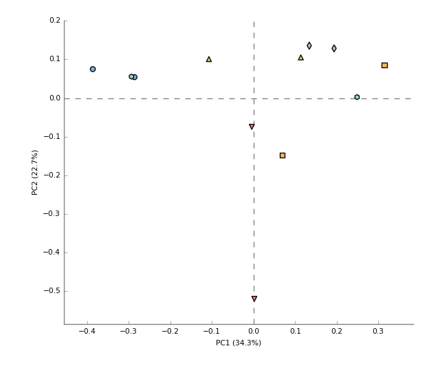
You may have noticed that a "Cancer" and "Normal" samples was taken from the same individuals. A pertinent question is whether these profiles are more similar simply because they are from the same individual. To investigate this, change the “Profile level” (top left) to “Genus”, ensure that the Group legend (top right) has been set to Individual, and that “PCA plot” has been set below the large middle window.

You should now be looking at a PCA plot that is coloured by which individual the samples came from (hit "Configure plot" to change settings):

images/mgs_tutorial_2017_images/MGS_tutorial_MetaPhlAn2_PCA.png

As you can see there is no obvious separation in the data points when coloured by individual - at the very least this isn't driving the major axes of variation.

Now change the group field (top right) to “Sample Type” and the PCA will be coloured according to that grouping instead.

Q7) How much of the variation is explained by PC3?

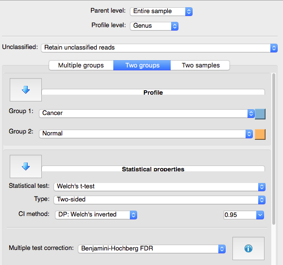
Now lets test what is significantly different between the groups at the Genus rank.

Under the “Two groups” dialog on the left, check that Welch's t-test is being used as the statistical test, and select “Benjamini-Hochberg FDR” for the multiple test correction.

images/mgs_tutorial_2017_images/metaphlan2_sampletype_stamp_settings.png

No genera are significantly different between samples based on sample type. This is likely at least partially due to the low sample sizes and low sequencing depths used for this tutorial. For the purposes of this tutorial we will focus on one genus that was significant before FDR correction. If we were to report this finding elsewhere we would need to clearly state the caveat that this genus was not significant after multiple-test corrections.

Q8) Which genus is significant based on its raw P-value?

Now lets look at a visualization of this genus.

Change the drop-down box that says "PCA plot" to "Box plot".

A new window will show a list of all the Genera. Select just the genus of interest to plot its relative abundance.

Q9) Save this boxplot by going to File -> Save plot...

In the next section we'll be reading in the HUMAnN2 output into STAMP - it's easier to close and reopen STAMP when reading in new files.

Analyzing a Subset of the HUMAnN2 output

Similar analyses can be run on the pathway abundances identified with HUMAnN2 as above. To begin with we can join all individual tables into a single table as above.

humann2_join_tables --input precalculated/humann2_out/ --file_name pathabundance --output humann2_pathabundance.tsv

Then we'll want to normalize each sample into relative abundance (so that the counts for each sample sum to 100).

humann2_renorm_table --input humann2_pathabundance.tsv --units relab --output humann2_pathabundance_relab.tsv

We could read this entire table (after running the reformatting commands below) and run similar analyses as we did above.

However, since HUMAnN2 yields functions stratified by taxa we could limit ourselves just to those functions that were found within the genus Streptococcus in order to focus on the above finding with the Metaphlan2 data. You could once again use grep to slice out only those pathways that are linked to this genus specifically.

In addition, more focused analyses could be based off of prior knowledge. For instance, pathways related to sugar degradation are especially of interest in the oral microbiome due to its relationship with dental health. We will test for differences between cancer and normal samples in STAMP similar to the earlier analysis based on this approach.

First an unstratified version of the pathway abundance table needs to be generated (the below command will also create a stratified version only in the same directory):

humann2_split_stratified_table --input humann2_pathabundance_relab.tsv --output ./

Then we can parse out the headerline and any lines matching the pathway of interest (LACTOSECAT-PWY: lactose and galactose degradation I).

head -n 1 humann2_pathabundance_relab_unstratified.tsv >> humann2_pathabundance_relab_LACTOSECAT-PWY.tsv
grep "LACTOSECAT-PWY" humann2_pathabundance_relab_unstratified.tsv >> humann2_pathabundance_relab_LACTOSECAT-PWY.tsv

Using sed to make string replacements we can also format the header-line for input into STAMP.

sed 's/_Abundance//g' humann2_pathabundance_relab_LACTOSECAT-PWY.tsv >  humann2_pathabundance_relab_LACTOSECAT-PWY.spf
sed -i 's/# Pathway/MetaCyc_pathway/' humann2_pathabundance_relab_LACTOSECAT-PWY.spf

Read file into STAMP as before with the mapping file.

Q10) Run a two-sided Welch's t-test between sample types for this pathway. What is the P-value?