CBW 2018 Metagenomic Taxonomic and Functional Composition Tutorial - LangilleLab/microbiome_helper GitHub Wiki
This tutorial is for Module 4 of the Canadian Bioinformatics Workshop running from June 5-7 2018 in Toronto.
Authors: Gavin Douglas and Morgan Langille
Table of Contents
- Introduction
- Pre-processing
- Generating stratified functional profiles with HUMAnN2
- Generating taxonomic profiles with contrasting approaches
- Next steps
Introduction
The main goal of this tutorial is to introduce students to a maker-based approach to taxonomic profiling (MetaPhlAn2) and to an approach for functional profiling (HUMAnN2). Throughout this tutorial we will emphasize that there is not a one-size-fits-all pipeline for analyzing MGS data. In particular, alternative approaches focusing on assembly and binning will be described in Module 5 of this workshop. Also, this tutorial doesn't give recommendations for how to run statistical tests on the data, which will be covered more in future modules. We'll be processing shotgun metagenomics data from the Inflammatory Bowel Disease Multi'omics database - at some points only 1 or 2 samples will be run through commands to save time.
Throughout this tutorial there will be questions that are meant to aid understanding. The answers are on this page, which you may want to open in a different tab.
Teaching objectives:
- Become familiar with raw shotgun metagenomics (MGS) data
- Learn how to use GNU Parallel to easily run commands on multiple files
- Learn common approaches to pre-process MGS data
- Learn how to generate stratified functional profiles from your MGS data with HUMAnN2 and basic ways to visualize this output
- Learn how to determine MGS taxonomic profiles using two contrasting approaches: (1) MetaPhlAn2 and (2) centrifuge
- Learn how to generate strain-level resolution output for MetaPhlAn2 output with StrainPhlAn
Bioinformatic tool citations
Properly citing bioinformatic tools is important to ensure that developers are getting the proper recognition. If you use any of the commands in this tutorial for your own work be sure to cite the relevant tools listed below!
- Bowtie2 (website, paper)
- centrifuge (website, paper)
- DIAMOND (website, paper)
- FASTQC (website)
- GNU Parallel (website, paper)
- HUMAnN2 (website, HUMAnN1 paper)
- kneaddata (website)
- MetaPhlAn2 (website, paper)
- Microbiome Helper (website, paper)
- MinPath (website, paper)
- RStudio (website)
- StrainPhlAn (website, paper) - Has a number of dependencies listed here
Activate conda environment
One common issue when trying to run StrainPhlAn, which is one of the tools we'll be using below, is that it's difficult to install! This is mainly due to a large list of dependencies and that it only works with an older version of samtools. Fortunately, these dependencies have already been installed in a conda environment (which was introduced in module 3).
You will need to activate this environment with this command:
source /usr/local/miniconda3/bin/activate spa
At the end of this tutorial you can exit the environment with this command:
source /usr/local/miniconda3/bin/deactivate
Introducing GNU Parallel
Often in bioinformatics research we need to run files corresponding to different samples through the same pipeline. You might be thinking that you can easily copy and paste commands and change the filenames by hand, but this is problematic for two reasons. Firstly, if you have a large sample size this approach will simply be unfeasible. Secondly, sooner or later you will make a typo! Fortunately, GNU Parallel provides a straight-forward way to loop over multiple files. This tool provides an enormous number of options: some of the key features will be highlighted below.
First copy over the test folder and enter it:
cp -r /home/ubuntu/CourseData/metagenomics/Module4/gnu_parallel_examples ./
chmod -R 755 gnu_parallel_examples
cd gnu_parallel_examples
Firstly, whenever you're using parallel it's a good idea to use the --dry-run option, which will print the commands to screen, but will not run them.
This command is a basic example of how to use parallel:
parallel --dry-run -j 2 'gzip {}' ::: example_files/fastqs/*fastq
This command will run gzip (compression) on the test files that are in example_files/fastqs/. There are 3 parts to this command:
- The options passed to GNU Parallel:
--dry-run -j 2. The-joption specifies how many jobs should be run at a time, which is 2 in this case. Again,--dry-runwill just print the commands to be run to the screen; this option needs to be removed when you actually want to run the commands! - The commands to be run:
'gzip {}'. The syntax{}stands for the input filename that is the last part of the command. - The files to loop over:
::: example_files/fastqs/*fastq. Everything after:::is interpreted as the files to read in!
Remove --dry-run from the above command and try running it again.
Sometimes multiple files need to be in given to the same command you're trying to run in parallel. As an example of how to do this, take a look at the paired-end FASTQ files in this example folder:
ls example_files/paired_fastqs/*fastq
The "R1" and "R2" in the filenames specify forward and reverse reads respectively. If we wanted to concatenate the forward and reverse files together we could use the below command:
parallel --dry-run -j 2 --link 'cat {1} {2} > {1/.}_R2_cat.fastq' ::: example_files/paired_fastqs/*R1.fastq ::: example_files/paired_fastqs/*R2.fastq
There are a few additions to this command:
- Two different sets of input files are given, which are separated by
:::(the first set is files matching *R1.fastq and the second set is files matching *R2.fastq). - The
--linkoption will allow files from multiple input sets to be used in the same command in order.{1}and{2}stand for a input file from the first and second set respectively. - Finally, the output file was specified as
{1/.}_R2_cat.fastq. The/will remove the full path to the file and.removes the extension.
It's important to check that each samples' files are being linked correctly when the commands are printed to screen with the --dry-run option. If the commands look ok then try running them without --dry-run now!
You can return to the higher directory with this command:
cd ..
Finally one thing to keep in mind when running slow command with parallel is that you can keep track of their progress (e.g. how many are left to run and the average runtime) with the --eta option.
Exploring the raw data
Alright now let's take a look at the data we'll be using for the main tutorial! The input files are FASTQ files, which contain information on the base-pairs in sequenced reads and the quality scores of each base-pair.
Eventually we'll take a look at 20 samples that are part of the Inflammatory Bowel Disease Multi'omics database. The basic metadata for these samples is in /home/ubuntu/CourseData/metagenomics/Module4/module4_metadata.txt.
For now we'll work with two example subsampled FASTQs, which are in this folder: /home/ubuntu/CourseData/metagenomics/Module4/raw_data.
Take a look with less at the forward ("R1") and reverse ("R2") reads. You'll see that there are 4 lines for each individual read. Also, note that in the forward and reverse FASTQs for each sample that the read ids (the 1st line for each read) are the same and in the same order (except for /1 or /2 at the end).
To find out how many reads are in each forward FASTQ we can simply take the line numbers. Since the files are gzipped we'll need to use zcat to uncompress them on the fly and pipe (|) this as input to the wc -l command, which will return the number of lines in plaintext files.
zcat /home/ubuntu/CourseData/metagenomics/Module4/raw_data/CSM79HR8_R1_subsampled.fastq.gz | wc -l
zcat /home/ubuntu/CourseData/metagenomics/Module4/raw_data/HSM7J4QT_R1_subsampled.fastq.gz | wc -l
Question 1: Based on the above line counts can you tell how many reads should be in the reverse FASTQs?
Pre-processing
Pre-processing is an important step when analyzing sequencing data. When not performed you could be allowing contaminants and/or low-quality reads to introduce noise to downstream analyses.
Visualizing read quality
A standard first step with pre-processing sequence data is to visualize the base-qualities over the reads along with other helpful statistics. FASTQC is a simple program that will allow you to explore this information!
You can FASTQC on the two test samples with this command (after making the output directory):
mkdir fastqc_out
fastqc -t 4 /home/ubuntu/CourseData/metagenomics/Module4/raw_data/*fastq.gz -o fastqc_out
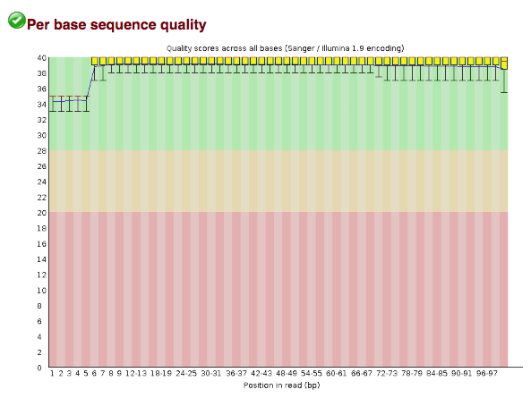
If you open one of output HTML files in your browser, you should see something like this under the per-base quality section:
images/CBW_2018/CSM79HR8_R1_fastqc_qual.png
These base qualities are not typical! Usually you would see the quality scores drop off near the end of the reads (and this tends to be even worse for reverse reads). However, it turns out that these reads have already been filtered! Importantly, this wouldn't have been obvious without visualizing the quality scores.
Filtering out low-quality reads
Even though these reads have already been through one round of quality filtering, we'll check them for contaminant sequences. Since these are human stool samples it's possible that there could be some human DNA that was sequenced (and could be high quality!). Also, sometimes PhiX sequences (a common sequencing control) aren't properly removed from output files. We'll want to remove both these types of sequences before proceeding.
We'll use kneaddata, which is a wrapper script for multiple pre-processing tools, to check for contaminant sequences. Contaminant sequences are identified by this tool by mapping reads to the human and PhiX reference genomes with Bowtie2. You would also typically trim trailing low-quality bases from the reads at this step with Trimmomatic, which kneaddata will do automatically if you didn't use skip-trim option below.
The below command will pass the read pairs to the same command, similar to how we ran them above. Note that in this case we're running 1 job at a time (-j 1) and each job is being run over 4 threads (-t 4). The Bowtie2 index files have already been made and are passed to the tool with this option: -db /home/ubuntu/CourseData/metagenomics/Module4/database_files/human_PhiX_bowtie2/GRCh38_PhiX.
parallel --eta -j 1 --link 'kneaddata -i {1} -i {2} -o kneaddata_out/ \
-db /home/ubuntu/CourseData/metagenomics/Module4/database_files/human_PhiX_bowtie2/GRCh38_PhiX \
-t 4 --bypass-trim' ::: /home/ubuntu/CourseData/metagenomics/Module4/raw_data/*_R1_subsampled.fastq.gz ::: /home/ubuntu/CourseData/metagenomics/Module4/raw_data/*_R2_subsampled.fastq.gz
If you take a peek in kneaddata_out you'll see that a number of output files have been created! The key information we want to know is how many reads were removed. This command will generate a simple count table:
kneaddata_read_count_table --input kneaddata_out --output kneaddata_read_counts.txt
Question 2: Take a look at kneaddata_read_counts.txt: how many reads in sample CSM79HR8 were dropped?
You should have found that only a small number of reads were discarded at this step, which is not typical. It happens that the developers of IBDMDB have provided the pre-processed data to researchers so it would have been strange to find many low-quality reads.
Question 3: It's reasonable that the processed data was provided by IBDMDB since their goal is to provide standardized data that can be used for many projects. However, why is it important that normally all raw data be uploaded to public repositories?
Let's enter the kneaddata output folder now and see how large the output files are:
cd kneaddata_out
ls -lh *fastq
In this example case the output files are quite small, but for typical datasets these files can be extremely large so you may want to delete the intermediate FASTQs if you're running your own data through this pipeline. Also, note that the output FASTQs are not gzipped - you could gzip these files if you planed on saving them long-term. In the meantime you can move the intermediate FASTQs to their own directory with these commands:
mkdir intermediate_fastqs
mv *_contam*fastq intermediate_fastqs
mv *unmatched*fastq intermediate_fastqs
cd ..
Generating stratified functional profiles
HUMAnN2 is a popular pipeline for profiling which genes and pathways could be active in a community based on shotgun metagenomics sequencing data. The two main phases of this pipeline are (1) mapping reads at the nucleotide-level to reference genomes of abundant organisms in your sample and (2) mapping the remaining reads at the protein level to a database of gene families.
Selecting a functional database
Before jumping in and using HUMAnN2 it's important to understand the differences between the possible databases you could use. You can see a list of these databases if you type this command:
humann2_databases
There are only two "chocoPhlAn" (nucleotide) databases, which makes it easy: a full database and a "DEMO" database only used for testing! The full database contains the reference genomes of common taxa that might be abundant in your samples. Reads are mapped to a subset of these genomes at the nucleotide alignment step!
It becomes more complicated when we consider which UniRef database should be used for the protein alignment step. Besides the DEMO database you should see these databases listed as options: uniref90_diamond, uniref50_diamond, uniref50_ec_filtered_diamond, uniref90_ec_filtered_diamond, and uniref50_GO_filtered_rapsearch2.
UniRef is a database of protein clusters at different identity levels. The number corresponds to at what sequence identity the sequences were clustered (e.g. UniRef90 proteins were clustered at 90%). These clusters are gene families - the idea is that the similar sequences will tend to have similar functions. However, the majority of UniRef gene families have unknown functions! The "filtered" databases are limited to only those gene families that have known functions based on Enzyme Classification (E.C.) numbers or Gene ontology (GO) information. These filtered databases are a lot smaller while still capturing most of the known functional information. The catch is that if you limit yourself to these databases you might be missing a key unknown function of interest!
Either way you would need to download and configure the database that you want to use for your own use (this has already been done for this tutorial).
Question 4: You can tell which database HUMAnN2 is configured to use by looking at the default values for --nucleotide-database and --protein-database when running humann2 --help. What are the default databases?
Question 5: If you were only interested in the abundances of higher-level functions would you expect different answers if you used the FULL UniRef90 database compared to the database limited to UniRef90 genes linked to E.C. numbers?
Running HUMAnN2
Now that we understand what databases HUMAnN2 can use, let's run it! HUMAnN2 (and MetaPhlAn2) don't use paired-end read information; the forward and reverse reads are mapped independently. To make the files easier to work with we can just concatenate the forward and reverse reads together since they'll be treated independently anyway.
Note the contaminated FASTQs must be removed before running the below command. You should check over the commands printed to screen to make sure the correct files are concatenated. Note that the forward and reverse reads are denoted by "_1" and "2" in the filenames due to how we ran kneaddata above - you can ignore the "R1" in the filenames.
concat_paired_end.pl -p 4 --no_R_match -o cat_reads kneaddata_out/*_paired_*.fastq
The forward and reverse reads will be concatenated into a single file per sample now in cat_reads/.
Question 6: What's a potential bias that could arise due to the forward and reverse reads being concatenated into the same file?
Running the full HUMAnN2 pipeline can take many hours on your personal computer with typical numbers of reads and samples. We'll just run the sample HSM7J4QT through the pipeline which will take ~3 minutes since it has been sub-sampled and we're using the DEMO protein database.
First we'll make a new folder to contain the HUMAnN2 output:
mkdir humann2_out
Now we'll run HUMAnN2 on sample HSM7J4QT. Note that a different nucleotide database is specified below to make the output more interesting. Also, we need to specify where the MetaPhlAn2 folder is so that the marker database can be located.
humann2 --threads 4 --input cat_reads/HSM7J4QT.fastq --output humann2_out/HSM7J4QT \
        --nucleotide-database /home/ubuntu/CourseData/metagenomics/Module4/database_files/humann2_databases/chocophlan/ \
        --metaphlan /usr/local/metaphlan2
Evaluating HUMAnN2 output
If you take a look in humann2_out you'll see that a folder has been created that contains all the output files. We'll take a closer look at some of these intermediate files in a moment. For now the key output files are (1) the abundance of gene families in a sample, (2) the abundance of pathways in a sample, and (3) the coverage of pathways in a sample. We'll take a look at these files one-by-one.
First take a look at the gene families abundance output file:
less humann2_out/HSM7J4QT/HSM7J4QT_genefamilies.tsv
The numbers in this file are the number of reads mapped to each gene family divided by the length of each gene family (in kilo-bases). The first line contains the number of UNMAPPED reads, which is the count of unaligned reads after both the nucleotide and protein alignment steps.
Question 7: What's the difference between the UNMAPPED and UniRef90_unknown categories?
Note that the abundance of each gene family is output in both stratified and unstratified output, which allows you to compare how different taxa are contributing functions in the community. Note: usually there will be many "unclassified" taxa that contribute functions. These correspond to cases where the gene was identified at the protein alignment stage only. These may be missing in the basic example considered here, but will be present in the files we'll be using below.
Question 8: Compare the abundance of UniRef90_D4JIP9 and UniRef90_A7UZW3 - can you tell whether more reads mapped to one of these gene families from this information alone?
Now take a look at the pathway abundance file:
less humann2_out/HSM7J4QT/HSM7J4QT_pathabundance.tsv
The format is very similar to the gene abundance file we looked at above, but now there is the additional UNINTEGRATED category. This category corresponds to gene families that aren't linked to particular pathways in the database. Again the output is in both stratified and unstratified output.
Question 9: The stratified counts summed to be equal to the unstratified counts in the gene families abundance file. Is that the case for the pathway abundance file? If not, why is that?
Now let's look at the pathway coverage output file:
less humann2_out/HSM7J4QT/HSM7J4QT_pathcoverage.tsv
The values in this file are similar to probabilities of where the pathway is present or not. In other words, if a pathway has coverage of 1 there is very high confidence that the pathway is present. This value is based on the proportion of enzymes that are required for a pathway that are present.
Question 10: Is it possible for a pathway to have high coverage even if it isn't detected in any individual species?
Now that we've taken a peek at the main output files let's check out the intermediate files that were created. There are a number of these files which are found in humann2_out/HSM7J4QT/HSM7J4QT_humann2_temp/.
There is a lot of information in this folder including how reads mapped to the custom Bowtie2 database and the MetaPhlAn2 output! There is also a logfile, which you should take a peek at:
less humann2_out/HSM7J4QT/HSM7J4QT_humann2_temp/HSM7J4QT.log
It's important to check what percent of reads were aligned at the nucleotide and protein alignment steps.
The Bowtie2 report of the overall alignment rate will look similar to this:
  50198 (100.00%) were unpaired; of these:
    28871 (57.51%) aligned 0 times
    17843 (35.55%) aligned exactly 1 time
    3484 (6.94%) aligned >1 times
42.49% overall alignment rate
You could quickly find this by searching for the string "overall alignment rate".
Similarly you can find the percent of unaligned reads at the protein alignment stage by searching for this string: "Unaligned reads after translated alignment".
Question 11: What percent of reads were unaligned at the protein alignment stage?
Basic visualizations of HUMAnN2 output
Running HUMAnN2 on many samples with millions of reads can take many hours (depending on many CPUs you have available). However, to give you a taste of what the full output looks like we have already run HUMAnN2 on 20 full samples (10 controls and 10 Crohn's disease) from the Inflammatory Bowel Disease Multi'omics Database rather than having you run them all! These output folders are in /home/ubuntu/CourseData/metagenomics/Module4/full_dataset/humann2_out/
To combine the final output files for each sample into a single table for the dataset you can run these commands (output to the humann2_final_out folder):
mkdir humann2_final_out

humann2_join_tables -s --input /home/ubuntu/CourseData/metagenomics/Module4/full_dataset/humann2_out/ --file_name pathabundance --output humann2_final_out/humann2_pathabundance.tsv
humann2_join_tables -s --input /home/ubuntu/CourseData/metagenomics/Module4/full_dataset/humann2_out/ --file_name pathcoverage --output humann2_final_out/humann2_pathcoverage.tsv
humann2_join_tables -s --input /home/ubuntu/CourseData/metagenomics/Module4/full_dataset/humann2_out/ --file_name genefamilies --output humann2_final_out/humann2_genefamilies.tsv
The above script humann2_join_tables knows to look only for files that have the matching string passed to the --file_name option.
Now let's try out visualization feature that HUMAnN2 provides out of the box! We'll focus on the pathway abundances for this analysis. Before starting we'll need to normalize each sample since they have different sequence depths.
This command will normalize the pathway abundances into copies per million (in each sample):
humann2_renorm_table -i humann2_final_out/humann2_pathabundance.tsv -u cpm -o humann2_final_out/humann2_pathabundance_relab.tsv
Many of the Huttenhower lab tools (such as HUMAnN2 and MetaPhlAn2) take "PCL" files in as input for data analysis. This is simply a table with samples as column and metadata and features (i.e. taxa and/or functions) as rows. You could format the input PCL file in a program like excel, but see some commands you can run in R to prepare this file:
# First read in the metadata file:
in_meta <- read.table("/home/ubuntu/CourseData/metagenomics/Module4/module4_metadata.txt", header=T, sep=" ", stringsAsFactors = FALSE)

# Set the rownames to be the sample labels
rownames(in_meta) <- in_meta$sample

# Transpose this table:
in_meta_t <- data.frame(t(in_meta), stringsAsFactors = FALSE)

# Now read in the pathway abundances (in copies per million):
in_path <- read.table("/path/to/humann2_final_out/humann2_pathabundance_relab.tsv", header=T, sep='\t', stringsAsFactors = FALSE, quote="", comment.char="", row.names=1)

# Remove "_Abundance" from the column names:
colnames(in_path) <- gsub("_Abundance", "", colnames(in_path))

# Order the sample columns to be the same as in the metadata table:
in_path <- in_path[,colnames(in_meta_t)]

# Combine these two tables by matching columns:
out_pcl <- rbind(in_meta_t, in_path)

# Write out this combined table of metadata and pathway abundances (note you'll need to change the path):
write.table(x = out_pcl, file = "/path/to/out/humann2_pathabundance_relab_meta.pcl", col.names=FALSE, row.names=TRUE, sep="\t", quote=FALSE)
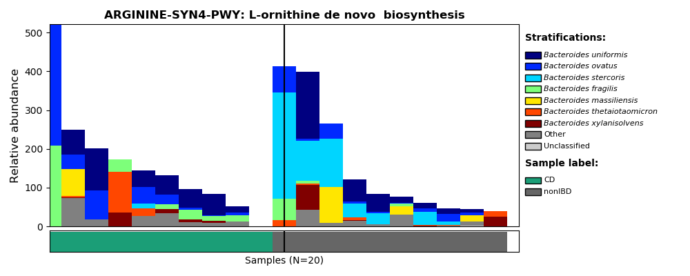
Now that we have created the correctly formatted input file (humann2_pathabundance_relab_meta.pcl) we can make basic visualizations. Below is the command to make a barplot for the ARGININE-SYN4-PWY: L-ornithine de novo biosynthesis pathway, with samples sorted by disease state and relative abundance. How much the top taxa are contributing to this function is also showed!
humann2_barplot --sort sum metadata --input humann2_pathabundance_relab_meta.pcl --focal-feature ARGININE-SYN4-PWY --focal-metadatum disease_state --last-metadatum disease_state --output ARGININE-SYN4-PWY_by_disease.png
The produced PNG should look like this:
images/CBW_2018/ARGININE-SYN4-PWY_by_disease.png
If there are pathways you are especially interested in this is a great way to explore the data! Even if there aren't particular pathways you're interested in it's a good idea to visualize a few pathways like this to make sure you understand the output and that it makes sense.
Generating taxonomic profiles with contrasting approaches
Now that we've taken a look at the basic out of functional profiling with HUMAnN2, let's move onto to taxonomic profiling!
Determining marker-based taxonomy with MetaPhlAn2
MetaPhlAn2 is a highly specific approach that identifies taxa based on known clade-specific marker genes. Fortunately, HUMAnN2 runs MetaPhlAn2 as one of the first step in the pipeline. Since we retained temporary files we can use this output without needing to re-run the tool over all samples.
Take a peak at the MetaPhlAn2 output produced for sample HSM7J4QT:
less -S humann2_out/HSM7J4QT/HSM7J4QT_humann2_temp/HSM7J4QT_metaphlan_bugs_list.tsv
You'll notice that the abundances are in relative abundances (they sum to 100 for each taxonomic level) and that all taxonomic levels from Kingdom to Strain (t__) are listed.
You can parse out particular taxa from this table easily with grep. For instance to parse out the lines for all strains you could type:
grep "t__" humann2_out/HSM7J4QT/HSM7J4QT_humann2_temp/HSM7J4QT_metaphlan_bugs_list.tsv
Adding the option -c to grep will return the number of lines that match that query.
Question 12: How many independent species (marked by s__) were identified by MetaPhlAn2?
Typically you would want to combine the output for all your samples. To merge the output from all the pre-calculated samples together you can use these commands. First, make a new output folder for each output command of HUMAnN2:
mkdir metaphlan2_out
cp /home/ubuntu/CourseData/metagenomics/Module4/full_dataset/humann2_out/*/*/*metaphlan_bugs_list.tsv metaphlan2_out/
Next merge these together into one file.
merge_metaphlan_tables.py metaphlan2_out/*metaphlan_bugs_list.tsv > metaphlan2_merged.txt
Finally, run the Linux tool sed to remove "_metaphlan_bugs_list" from the column names of this file.
sed -i 's/_metaphlan_bugs_list//g' metaphlan2_merged.txt
Question 13: How many independent species are there in this file?
You now have a table of MetaPhlAn2 taxa abundances for all the samples with taxa as rows and samples as columns.
Question 14: Similar to HUMAnN2, you can pass options to MetaPhlAn2 that will be used by Bowtie2. Why would you expect more false positives if Bowtie2 was run with the --local option?
Binning approach teaser: centrifuge
Above we found very few species with MetaPhlAn2, which is partially due to the low sequencing depth in the example FASTQ we ran through HUMAnN2. However, it's important to realize that since MetaPhlAn2 is a marker-based approach it will often only identify relatively few species in your data. In contrast, binning approaches tend to have the opposite approach: they'll return a lot of false positives!
To hammer home this point you can run one representative binning approach known as centrifuge to taxonomically profile the same sample we were inspecting above. You can run centrifuge with this command (note that it reads in forward and reverse FASTQs separately):
mkdir centrifuge_out

centrifuge -p 4 --mm -x /home/ubuntu/CourseData/metagenomics/Module4/database_files/centrifuge_index/p_compressed+h+v -1 kneaddata_out/HSM7J4QT_R1_subsampled_kneaddata_paired_1.fastq -2 kneaddata_out/HSM7J4QT_R1_subsampled_kneaddata_paired_2.fastq -S centrifuge_out/HSM7J4QT_out.txt --report-file centrifuge_out/HSM7J4QT_report.txt
centrifuge outputs 2 key files which were specified in the above command. Take a look at the report file:
less centrifuge_out/HSM7J4QT_report.txt
This file is the summary of the centrifuge output. The first line of this file describes what each column contains. One thing that will jump out right away is that the taxa tend to be called by very few reads. The centrifuge authors rely on the user to process the output; for instance taxa called by a single read are not reliable! There are further filtering suggestions on the centrifuge website.
Question 15: How many species of Bacteroides were identified in the subsampled HSM7J4QT sample by centrifuge? By MetaPhlAn2?
Question 16: What is the abundance of Dialister invisus in the MetaPhlAn2 and centrifuge outputs for sample HSM7J4QT?
Neither of these questions are meant to suggest that either tool is better than the other. In fact, in these cases we can't be sure which tool's output was more correct anyway. Instead you should think about what tool would be best for your data while acknowledging that the output wont be perfect!
Strain-level profiling based on MetaPhlAn2 output
There is growing interest in profiling how exact strains are distributed across samples. StrainPhlAn is a tool which will identify strains based on shared variants in the sequences match marker genes. There are mainly possible applications of MetaPhlAn2 and StrainPhlAn, but here we'll focus on profiling Bacteroides ovatus strains. Bacteroides ovatus is a gut commensal that has in at least one paper been reported to cause antibody responses in IBD patients (Saitoh et al. 2002). It turns out that this species is present in almost all of the samples based on the MetaPhlan2 output. It's possible that particular strains of Bacteroides ovatus elicit immune responses between Crohn's disease and control subjects; below we'll use StrainPhlAn to test this hypothesis!
This tool requires MetaPhlAn2 output files. Although MetaPhlAn2 was run above, StrainPhlAn requires the SAM-formatted file of read mappings output by MetaPhlAn2 along with the default taxonomic profile. Running these commands on all 20 samples would be time-consuming, but you should run the below commands on a single sample to know how they work.
Now create a folder for the example output file:
mkdir example_strainphlan2_out
Now re-run MetaPhlAn2 and output the SAM file containing the exact read mappings.
metaphlan2.py cat_reads/CSM79HR8.fastq example_strainphlan2_out/CSM79HR8_profile.txt --bowtie2out example_strainphlan2_out/CSM79HR8_bowtie2.txt --samout example_strainphlan2_out/CSM79HR8.sam.bz2 --input_type fastq --bowtie2db /usr/local/metaphlan2/db_v20/ --nproc 4
The SAM file was written out in compressed format to example_strainphlan2_out/CSM79HR8.sam.bz2. The bulk of this file contains information on where each read aligned, at what orientation, and how well the reads mapped.
Question 17: The above command ran MetaPhlAn2 on a single sample's FASTQ file. How would this command look if you re-wrote it to be run over all FASTQs in cat_reads/ with parallel?
Now that we have the SAM file which links individual reads mapped to marker genes we can run sample2markers.py, which will determine the consensus of unique marker genes for each species in the sample. At later steps these consensus sequences will be used for identifying single-nucleotide polymorphisms (i.e. mutations) that can differentiate strains.
sample2markers.py --ifn_samples example_strainphlan2_out/CSM79HR8.sam.bz2 --input_type sam --output_dir example_strainphlan2_out/ --nproc 4
Since in this example we're interested in specifically comparing strains of Bacteroides ovatus we can extract the markers specifically for this species with the below command, which will be written to s__Bacteroides_ovatus.fasta.
extract_markers.py --mpa_pkl /home/ubuntu/CourseData/metagenomics/Module4/database_files/db_v20/mpa_v20_m200.pkl --ifn_markers /home/ubuntu/CourseData/metagenomics/Module4/database_files/db_v20/mpa_v20_m200.fna --clade s__Bacteroides_ovatus --ofn_markers s__Bacteroides_ovatus.fasta
Finally we can run the main StrainPhlAn function which will output a number of files including the phylogenetic tree with the distances between strains of Bacteroides ovatus.
strainphlan.py --ifn_samples /home/ubuntu/CourseData/metagenomics/Module4/full_dataset/strainphlan2_out/*.markers --ifn_markers s__Bacteroides_ovatus.fasta --output_dir . --clades s__Bacteroides_ovatus --marker_in_clade 0.2
The best tree outputted by RAxML was written to RAxML_bestTree.s__Bacteroides_ovatus.tree, which is written in newick format.
Visualizing this tree is the best way to evaluate the StrainPhlAn output, which we'll do in RStudio.
Once you have RStudio open you can load the two required libraries with these commands, which need to be run in R:
library(ggplot2)
library(ggtree)
ggtree is a useful package for annotating and visualizing trees. ggplot2 is a general purpose visualization package which is widely used when analyzing data with R.
Next we'll read in the output newick treefile and the metadata that links each sample id to whether they have Crohn's disease or are control subjects. Note that you may need to change the paths to the files below (you can get your current working directory on the command-line by typing pwd).
in_meta <- read.table("/home/ubuntu/CourseData/metagenomics/Module4/module4_metadata.txt",
                      header=T, sep=" ", stringsAsFactors = FALSE)

bovatus_tree <- read.tree("/path/to/RAxML_bestTree.s__Bacteroides_ovatus.tree")
To use the ggtree package you need to convert the tree object to a special object with this command. We'll do that below and add the metadata that we read in to this tree as well.
bovatus_gg <- ggtree(bovatus_tree)
bovatus_gg <- bovatus_gg %<+% in_meta
Question 18: The class function in R is useful for knowing what types of objects you're using. What classes of object are bovatus_tree and bovatus_gg? Note: you can see the descriptions of R functions by typing a question mark before the function name, for example: ?class.
Finally let's plot the tree with this command:
bovatus_gg +
  geom_tippoint( size = 3, aes( color = disease_state ) ) +
  aes( branch.length = 'length' ) +
  theme_tree2() + theme(legend.position="right")
Question 19: Does this tree support the hypothesis that different strains of B. ovatus are found in Crohn's disease and control subjects?
Next steps
Hopefully this tutorial has introduced you to some useful tools which you can apply to your own shotgun metagenomics data! However, keep in mind that although these tools are popular that there are many other tools available to explore (including more binning and assembly methods introduced in a later module!). It's important to consider which approach would be best for your data and/or research question.
If you still have time you can look into a few downstream tools which you could use for analyzing the above output files. For instance LefSe is a tool developed to identify significant taxa or functions between groups. You might also be interested in BURRITO, which enables users to explore taxa-function relationships in stratified output files (e.g. the HUMAnN2 output files) through nice visualizations.