Normalized count analysis - Kan-E/RNAseqChef GitHub Wiki

Normalized count analysis identifies similar samples and gene expression patterns using clustering methods.
By uploading the gene list, you can extract only the count data of the gene of interest and then perform clustering analysis.
k-means clustering identifies the gene groups that show similar expression patterns.

The input format for normalized count analysis is the same as for pair-wise DEG and 3 conditions DEG.
If you have read the description of pair-wise DEG or 3 conditions DEG, you do not need to read the below.

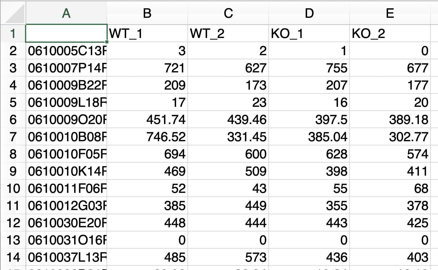
The analysis can only be performed with raw count data if the following conditions are fulfilled:

- The replication number is represented by the underline “_”.
- Do not use the underline "_" for anything else. 

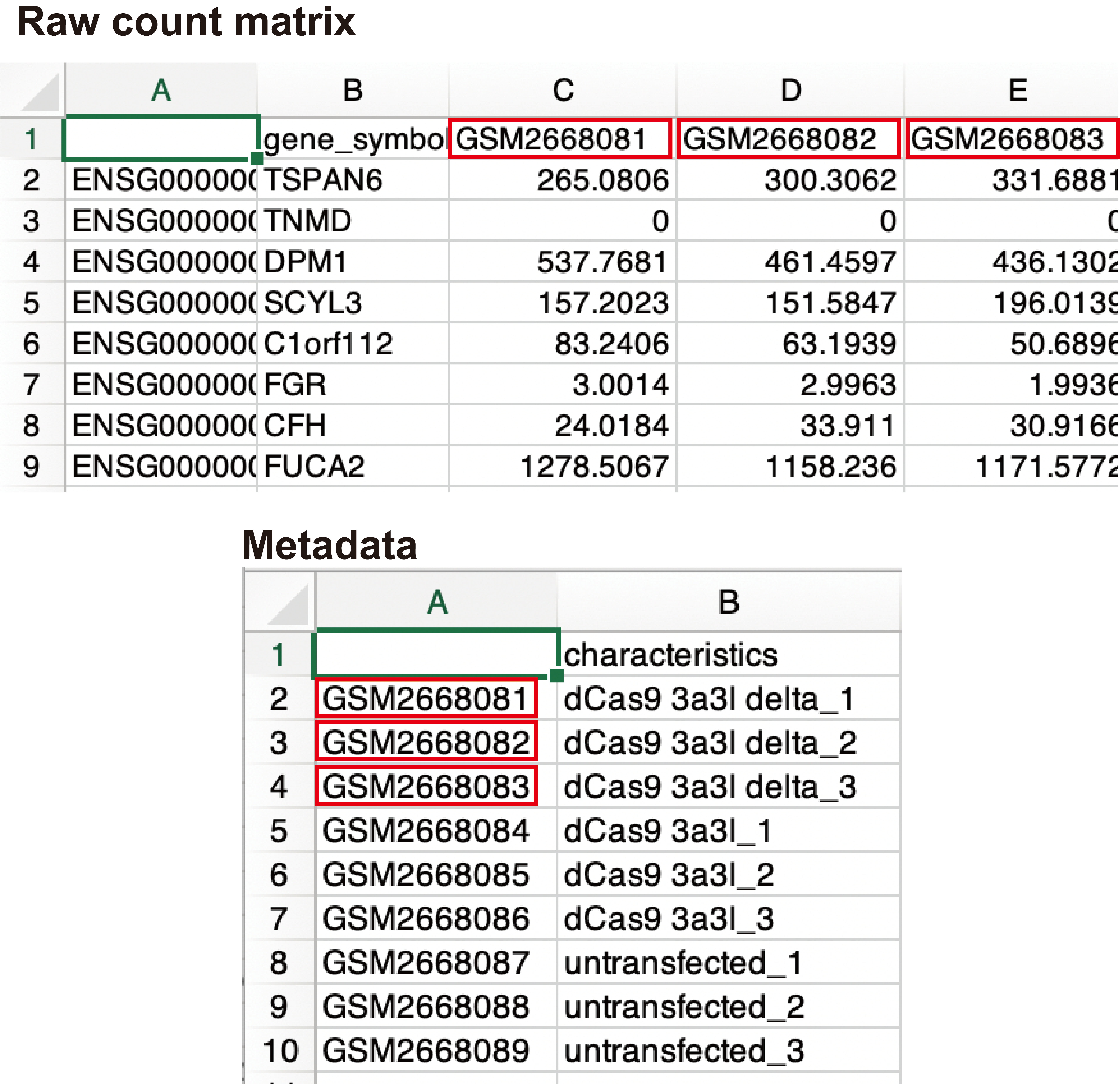
This format can be used if the above conditions are not fulfilled, for example, if the sample name is an accession number, or if the raw count data contain extra information that is not the subject of analysis.
Metadata must contain the following information:

- The first column is the sample names used in the raw count data.（e.g., accession number）
- The second column is the corresponding sample name that matches the sample name in the first column. (e.g. Control_1)
- The third and subsequent columns do not affect the analysis.

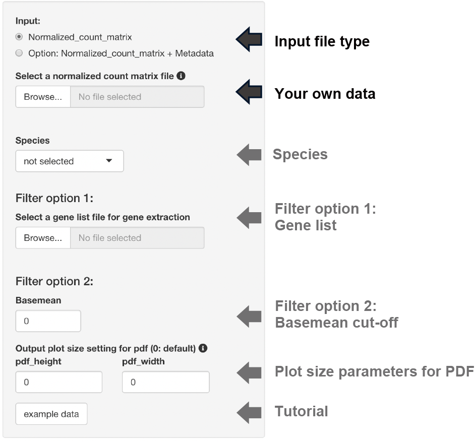
The following analysis is performed by selecting the dataset species.

- Conversion to gene symbols if the gene name is ENSEMBL ID

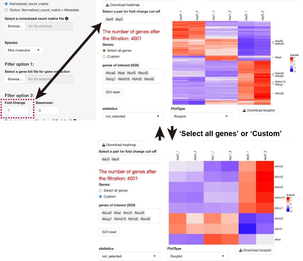
When the gene list was uploaded, clustering analysis of the normalized count data is performed after gene extraction with the gene list.

The base mean threshold can be set.

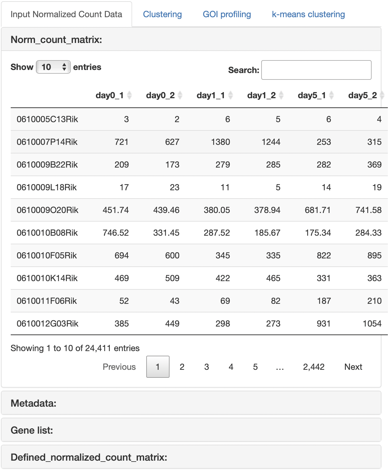
The uploaded files are displayed.
In the case that metadata and gene list are uploaded, it also show the normalized count data that is re-defined with metadata and gene list.

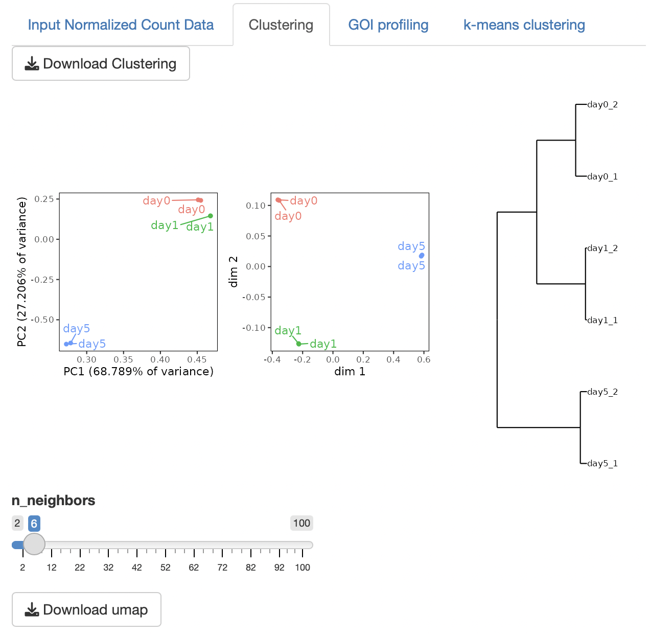
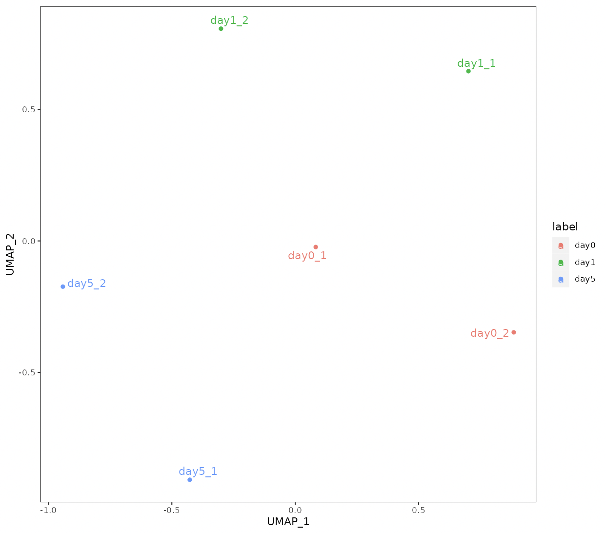
Four types of clustering analyses are performed: principal component analysis (PCA), multidimensional scaling (MDS), hierarchical clustering with ward.D2, and UMAP (uniform manifold approximation and projection).

n_neighbors in UMAP control how UMAP balances the local versus global structure in the data.
Low values of n_neighbors force UMAP to concentrate on very local structures, whereas large values push UMAP to look at the larger neighborhoods of each point.
In the case of a small number of samples, n_neighbors should be small.

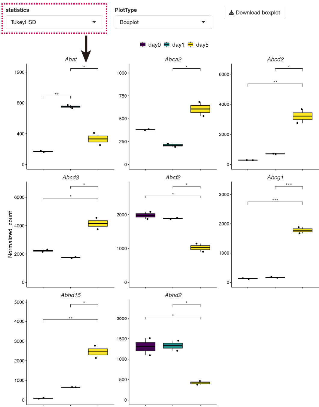
The heatmap and boxplot of the genes selected from the GOI list are displayed.

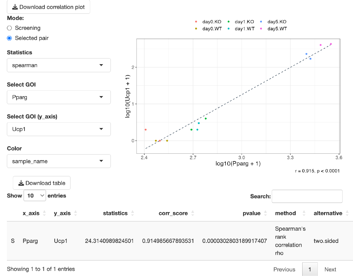
Correlation analysis is performed.
There are two modes available.

This mode displays a correlation plot for two genes of interest. You can select genes from both Select GOI and Select GOI (y_axis). The color of the dots can be chosen from the Color option. If 'Sample name' is selected, the dots will be colored by groups. If 'Gene name' is chosen, they will be colored based on the expression levels of the selected genes, with blue representing low expression and red indicating high expression.

You can also choose between 'Spearman’s rank correlation analysis' and 'Pearson’s correlation analysis' as the method for Correlation analysis from the Statistics.

This function calculates the correlation coefficients between genes of interest and all parameters present in the count data.

• Select the gene of interest (Bait) from Select GOI.
• Click Start to execute the analysis. As a result, you will obtain a correlation rank plot where the vertical axis represents correlation coefficients, and the horizontal axis represents the rank of correlations (in descending order). Genes showing positive and negative correlations will be identified based on the padj (or pval) cut-off value. The padj value is calculated using the BH method.

Clicking on a gene of interest in the table data will display a correlation plot with the selected gene as the Bait. While it's not possible to display correlation plots for all selected genes within the browser, you can obtain all the graphs by clicking Download correlation plot (all genes from 'select GOI').

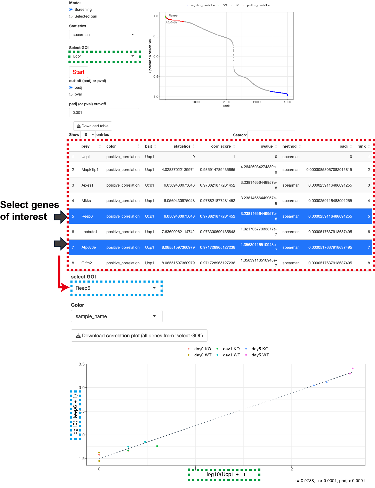
Furthermore, you can select multiple prey genes at once by enclosing the area of interest with a rectangle on the correlation rank plot. To obtain all the graphs simultaneously, simply click on Download correlation plot (all genes from 'select GOI').

k-means clustering is performed.
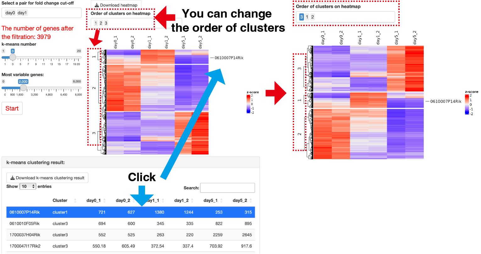
Select a pair for fold change cut-off: You can choose the condition pair for which you want to apply the Cut-off based on Fold Change.
The number of clusters: You can adjust the number of clusters using the slider.
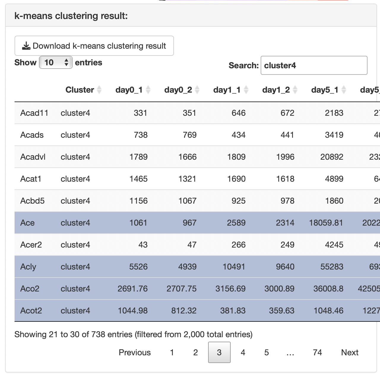
To optimize server memory usage, the analysis is limited to a specific number of genes, focusing on the Most variable genes. If you want to analyze all genes after the FoldChange cut-off, please specify a number higher than what is displayed in The number of genes after the filtration under Most variable genes. The results of the k-means clustering is presented in the k-means clustering result panel, including a table showing the correspondence between genes and clusters.
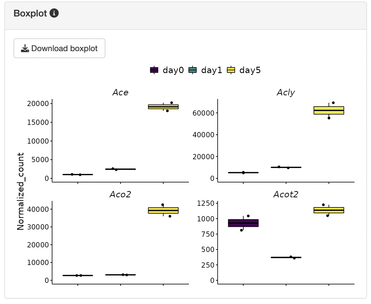
Clicking on genes of interest will display their positions on the heatmap, along with a box plot for the selected genes.
Additionally, you can modify the order of clusters on the heatmap by using the Order of clusters on heatmap control.