ChIP AP Outputs - mbassalbioinformatics/ChIP-AP GitHub Wiki
-
Acquisition of raw sequencing files. ChIP-AP can directly process demultiplexed FASTQ, or compressed FASTQ (.gz) format sequencing files. ChIP-AP can also process aligned reads in BAM format (which bypasses QC & Filtering and Alignment stages of the pipeline and proceeds directly to Peak Calling & Merging). Reads may be single or paired ends. Background control is compulsory, no unmatched samples allowed here. For background, Input control is the commonly accepted standard and not IgG controls.
-
Sample recognition and registration. Performed by the main script. Each input sample is registered into the system and given a new name according to their sample category (ChIP or background control), replicate number, and whether it’s the first or second read (in case of paired end sequencing data). Afterwards, their format and compression status is recognized and processed into gun-zipped FASTQ as necessary.
-
Generation of multiple modular scripts. Each stage of analysis in ChIP-AP is executed from persistent individually generated scripts. This was an intentional design decision as it allows for easy access for debugging and modifications of any step within the pipeline without hunting through the master ChIP-AP scripts; simply re-run the troublesome step to figure out what’s going on or swap it out entirely if you really want. You can thank us later if you have to modify and tailor something later and don’t have to drudge through the trenches of someone else’s code. Chocolate treats always welcome!
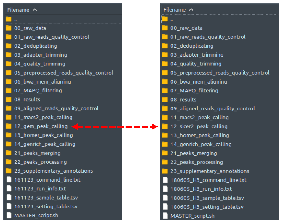
How does it look like? After this step is done (which is the end of your ChIP-AP processes if you don’t use the “--run” flag to run the pipeline immediately), you can see within your designated output directory a single folder named as per your “--setname” input, with contents as shown below regardless of single-end or paired end-mode:
The left figure shows a dataset with narrow peak type, while the right figure shows a dataset with broad peak type. Note that the peak calling module – folder number 12 – is interchangeable between GEM for narrow peak type and SICER2 for broad peaks. This is because of the significant difference between these 2 peak callers in handling the respective datasets. GEM does a great job for TF’s and SICER2 for broad peaks.
Each of these folders are basically empty, and contains a script which is named based on the folder name (e.g., script 02_deduplicating.sh inside folder 02_deduplicating). Each of these scripts will be executed in numerical sequence when you run the pipeline. Aside from these scripts, there will be several miscellaneous text files which contain essential information of your pipeline run (See Miscellaneous Pipeline Output section below for details). Lastly, there is your big red button: the MASTER_script.sh that you can simply call (if you did not use the “--run” flag when calling ChIP-AP) to sequentially run all the scripts within the aforementioned folders.
-
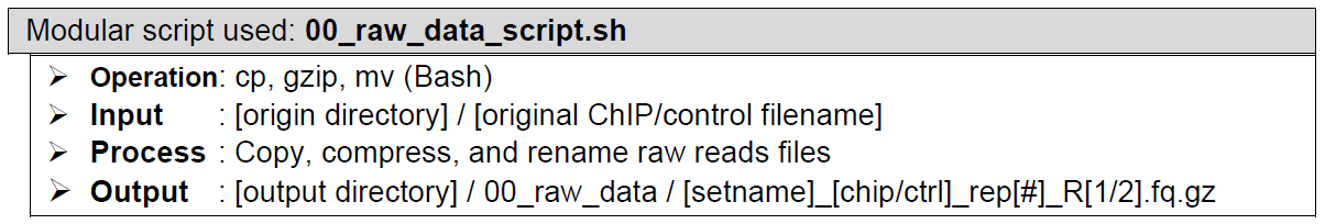
Copying, compressing, and renaming of the raw sequencing reads. In the very beginning, ChIP-AP makes (in the user-designated output folder) a copy of each unaligned sequence reads file, compresses them into a gunzipped file (if not already), and renames them with the prepared new name from step “2. Sample recognition and registration”. If the given inputs are aligned reads (bam files), the pipeline starts at step “12. Sorting and indexing of aligned reads files” (see below) and the copying and renaming are taken over by 08_results_script.sh where the original bam files are directly sorted and the pipeline proceeds normally from there.
How does it look like? After 00_raw_data_script.sh had been executed, all reads files in your dataset will have been copied into this folder: 00_raw_data, compressed into fq.gz, and renamed into something like the preview below, regardless of your initial filenames, fastq formatting or extensions.
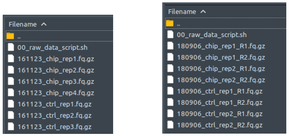
The left figure shows a single-end dataset with four ChIP samples and three control samples. The right figure shows a paired-end dataset with two ChIP samples and two control samples, in which every sample consists of two files: the first read (R1), and the second read (R2).
All these fq.gz files will be immediately deleted at the end of 02_deduplicating_script.sh execution if “--deltemp” flag is used when calling ChIP-AP. We won’t explain how to open and read these fq.gz files, since if you need us to tell you that, you most probably won’t be able to understand the contents of the files anyway.
-
Raw sequencing reads quality assessment. Performed by FastQC. Reads quality assessment is performed to check for duplicates, adapter sequences, base call scores, etc. Assessment results are saved as reports for user viewing. If the final results are not as expected, it’s worthwhile to go through the multiple QC steps and track the quality of the data as its processed from this folder onwards. If the default QC steps aren’t cleaning up the data adequately, you may need to modify some parameters to be more/less stringent with cleanup. From our testing, our default values seem to do a fairly adequate job though for most datasets. They even work pretty well for RNA-Seq and RIP-Seq datasets too!
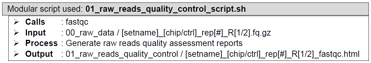
How does it look like? After 01_raw_reads_quality_control_script.sh had been executed, the folder: 01_raw_reads_quality_control will contain all these quality assessment reports for every raw reads file in folder 00_raw_data, just like below:
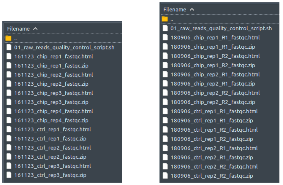
The left figure shows a single-end dataset with four ChIP samples and three control samples. The right figure shows a paired-end dataset with two ChIP samples and two control samples, in which every sample consists of two files: the first read (R1), and the second read (R2).
The .zip files contains the individual components to be compiled for the report so you can ignore those. To read the reports, open the .html files in your web-browser of choice (Safari, Edge, Firefox). This file is a multitabular file in which you can evaluate the quality of your experiment, sequencing, etc. Comprehensive as it is, explaining the contents in detail would take a whole new guide by itself. Therefore, its best to check out the documentation of the developers for all the details: https://www.bioinformatics.babraham.ac.uk/projects/fastqc/Help/.
-
Deduplication of reads. Performed by clumpify from BBMap package. Clumpify is used to remove optical duplicates and tile-edge duplicates from the reads file in addition to PCR duplicates. This step is performed in preference to a PCR deduplication step downstream. Optimization of file compression is also performed by clumpify during deduplication process, in order to minimize storage space and speed up reads file processing. Clumpify will also ensure your processed files are output in PHRED33 format so as to not break any down-stream program processing. Also, if there are ill-formatted reads (if using publicly available dataset) then Clumpify will also attempt to fix these reads.
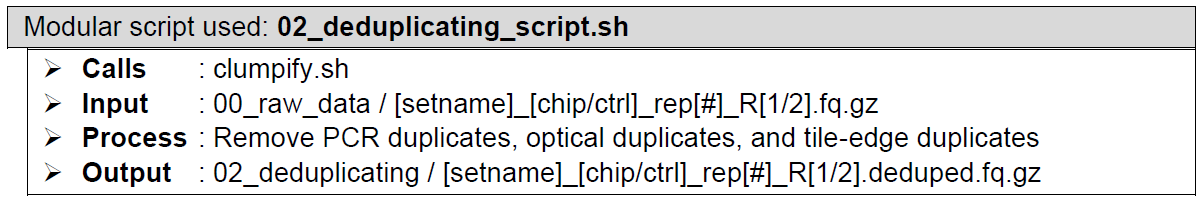
How does it look like? After 02_deduplicating_script.sh had been executed, the folder: 02_deduplicating will contain all these deduplicated reads files (marked by the extension: .deduped.fq.gz), just like below:
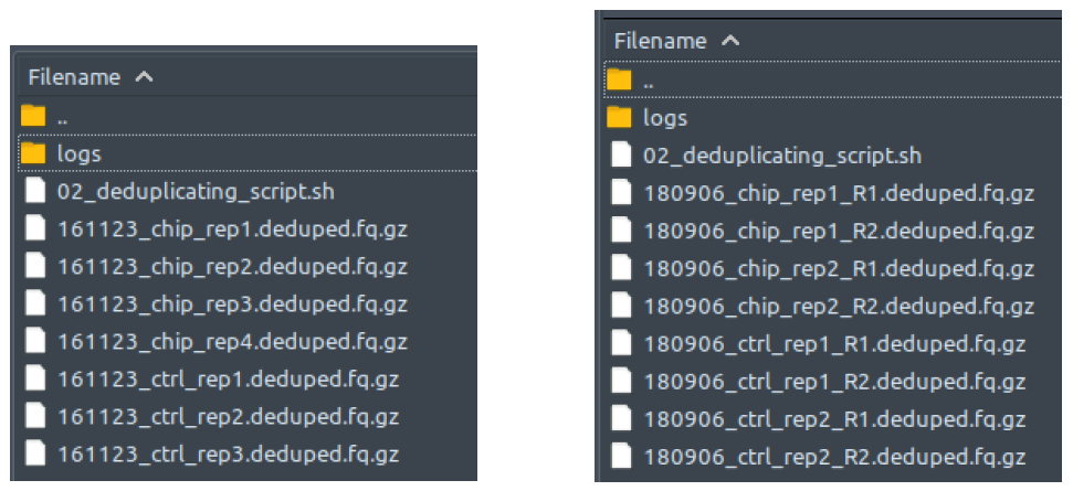
The left figure shows a single-end dataset with four ChIP samples and three control samples. The right figure shows a paired-end dataset with two ChIP samples and two control samples, in which every sample consists of two files: the first read (R1), and the second read (R2).
There should be one deduplicated file for each processed raw reads file from folder 00_raw_data. Paired-end files are processed in pairs by clumpify. All these deduped fq.gz files will be deleted at the end of 02_deduplicating_script.sh execution if “—deltemp” flag is used on ChIP-AP call.
-
Adapter trimming of reads. Performed by BBDuk from BBMap package. BBDuk scans every read for adapter sequences in its reference list of adapter sequences. The standard BBDuk adapter sequence reference list ‘adapter.fa’ is used as the default in the pipeline. Any sequencing adapter present in the reads is removed. Custom adapter sequence can be used whenever necessary by modifying the adapter.fa file and adding your new sequences. Just remember to make a backup of the original yeah? We warned you!
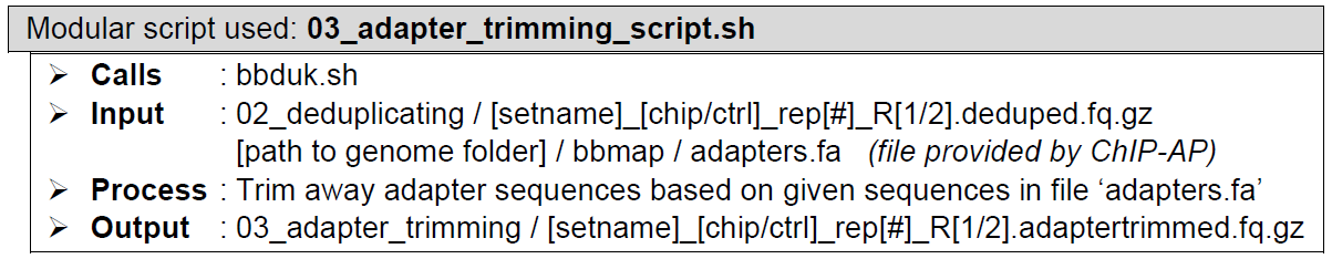
How does it look like? After 03_adapter_trimming_script.sh had been executed, the folder: 03_adapter_trimming will contain all these adapter-trimmed reads files (marked by the extension: .adaptertrimmed.fq.gz), just like below:
The left figure shows a single-end dataset with four ChIP samples and three control samples. The right figure shows a paired-end dataset with two ChIP samples and two control samples, in which every sample consists of two files: the first read (R1), and the second read (R2).
There should be one adapter-trimmed file for each processed deduplicated reads file from folder 02_deduplicating. Paired-end files are processed in pairs by bbduk. All these adaptertrimmed.fq.gz files will be automatically deleted at the end of 3_adapter_trimming_script.sh execution if “--deltemp” flag is used on ChIP-AP call.
-
Quality trimming of reads. Performed by Trimmomatic. Trimmomatic scans every read and trims low quality base calls from the ends of the reads. Additionally, it scans with a moving window along the read and cuts the remainder of the read when the average quality of base calls within the scanning window drops below the set threshold. Finally, it discards the entirety of a read of it gets too short post-trimming for alignment to reference genome, minimizing the chance of reads being multi-mapped to multiple genomic locations. Check out the settings table for the parameters used. Some value changes won’t make a big difference to the output, some will make a huge difference, so careful what you set this to.
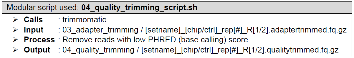
How does it look like? After 04_quality_trimming_script.sh had been executed, the folder: 04_quality_trimming will contain all these quality-trimmed reads files (marked by the extension: .qualitytrimmed.fq.gz), just like below:
The left figure shows a single-end dataset with four ChIP samples and three control samples. The right figure shows a paired-end dataset with two ChIP samples and two control samples, in which every sample consists of two files: the first read (R1), and the second read (R2).
There should be one quality-trimmed file for each processed adapter-trimmed reads file from folder 03_adapter_trimming. Paired-end files are processed in pairs by trimmomatic. Unpaired reads are separated (saved into unpaired.fq.gz files) from the paired reads (saved into qualitytrimmed.fq.gz files). Only the paired read (extension: .qualitytrimmed.fq.gz) are processed further in the pipeline. All these qualitytrimmed.fq.gz and unpaired.fq.gz files will be immediately deleted at the end of 04_quality_trimming_script.sh execution if “--deltemp” flag is used on ChIP-AP call.
-
Pre-processed reads quality assessment. Performed by FastQC. Quality assessment is performed to check for the efficiency of cleanup. Results are saved as reports.
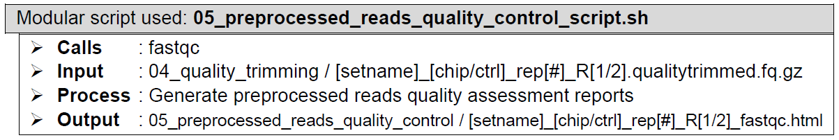
How does it look like? After 05_preprocessed_reads_quality_control_script.sh had been executed, the folder: 05_preprocessed_reads_quality_control will contain all these quality assessment reports for every qualitytrimmed.fq.gz file in folder 04_quality_trimming, just like below:
The left figure shows a single-end dataset with four ChIP samples and three control samples. The right figure shows a paired-end dataset with two ChIP samples and two control samples, in which every sample consists of two files: the first read (R1), and the second read (R2).
The .zip files contains the individual components to be compiled for the report so you can ignore those. To read the reports, open the .html files in your web-browser of choice (Safari, Edge, Firefox). This file is a multitabular file in which you can evaluate the quality of your experiment, sequencing, etc. Comprehensive as it is, explaining the contents in detail would take a whole new guide by itself. Therefore, its best to check out the documentation of the developers for all the details: https://www.bioinformatics.babraham.ac.uk/projects/fastqc/Help/.
-
Reads alignment to reference genome. Performed by the mem algorithm in BWA aligner. The appropriate genome reference for the sample is given as a command line argument. The default genome reference is hg38. Precomputed genome references for hg38, hg19, mm9, mm10, dm6, and sacCer3 are downloaded as part of the ChIP-AP installation process. Tutorials for custom / different genome references can be found on the ChIP-AP GitHub (coming soon!). BWA is used in preference to other aligners such as Bowtie2 as in benchmarking papers (Thankaswamy-Kosalai et al., 2017), we were more satisfied with the results of BWA, hence its inclusion in this pipeline.
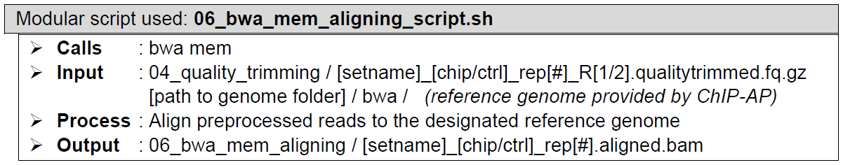
How does it look like? After 06_bwa_mem_aligning_script.sh had been executed, the folder: 06_bwa_mem_aligning will contain all these aligned reads files (marked by the extension: .aligned.bam), just like below:
The left figure shows a single-end dataset with four ChIP samples and three control samples. The right figure shows a paired-end dataset with two ChIP samples and two control samples. Note that right here the first reads (R1), and the second reads (R2) had both been aligned into the same reference genome, and thus no longer separated in two different files. Paired-end files are processed in pairs by bwa mem.
There should be one aligned reads file here for each processed single-end, or for every two processed paired-end quality-trimmed reads file from folder 04_quality_trimming. All these aligned.bam files will be deleted at the end of 06_bwa_mem_aligning_script.sh execution if “--deltemp” flag is used on ChIP-AP call.
-
Alignment score quality filtering. Performed by samtools view. This filter (if set) will remove all reads with alignment score (MAPQ) below a user defined threshold. Reads with suboptimal fit into the genome and/or reads with multiple ambiguous mapped locations can easily be excluded from the reads file using this filter step also. To disable MAPQ filtering, simply remove all flags from the settings table for this step. As for what is an appropriate filter to set? There are many blog posts by bioinformaticians talking about MAPQ inconsistency and what the scores mean, so that discussion is a long one to have. Basically, we have 2 takes on the matter, if you want to include everything, then remove the parameters for this step from the settings table. If you want to be relatively stringent then use the default MAPQ filter of 20.
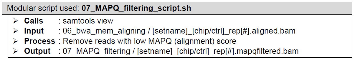
How does it look like? After 07_MAPQ_filtering_script.sh had been executed, the folder: 07_MAPQ_filtering will contain all these MAPQ-filtered reads files (marked by the extension: .mapqfiltered.bam), just like below:
The left figure shows a single-end dataset with four ChIP samples and three control samples. The right figure shows a paired-end dataset with two ChIP samples and two control samples. Again, note that right here the first reads (R1), and the second reads (R2) had both been aligned into the same reference genome by bwa mem in above, and thus no longer separated in two different files.
There should be one MAPQ-filtered reads file here for each processed aligned reads file from folder 06_bwa_mem_aligning. All these mapqfiltered.bam files will be deleted at the end of 07_MAPQ_filtering_script.sh execution if “--deltemp” flag is used on ChIP-AP call.
-
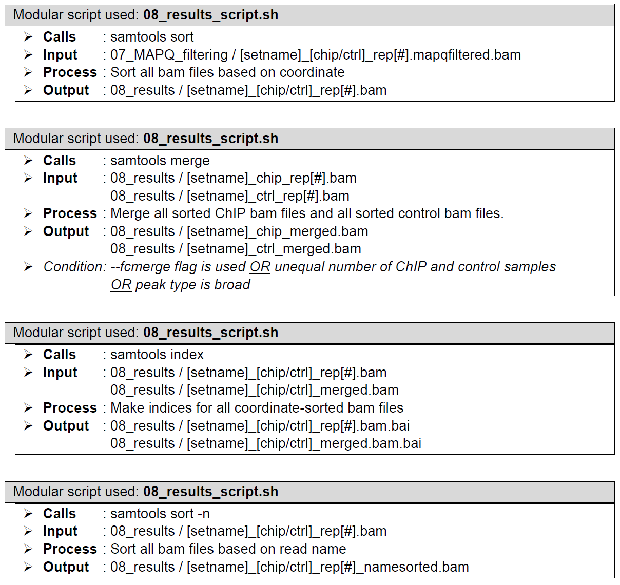
Sorting and indexing of aligned reads files. Performed by samtools sort and samtools index, which do nothing to the aligned reads files other than sorting and indexing, priming the aligned reads files for further processing.
How does it look like? Detailed output preview of step 12, 13, and 14 are combined below step 14
-
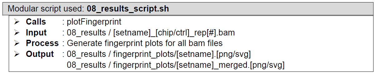
ChIP pulldown efficiency assessment. Performed by plotFingerprint from the deeptools package, which generates fingerprint plots. These serve as a quality control figure that shows DNA pulldown efficiency of the ChIP experiment. Refer to the appropriate documentation for full details but in short – the input should be as close to the 1:1 diagonal as possible and the better enrichment seen in your sample, the more its curve will bend towards the bottom right. You want (ideally) a large gap between the chip and the control samples. PNG files are provided for easy viewing, SVG files provided if you want to make HQ versions later for publication.
How does it look like? Detailed output preview of step 12, 13, and 14 are combined below step 14
-
Visualization track generation of aligned reads files. Performed by bamCoverage from the deeptools package. Generates bigwig files for quick and simple visualization of reads distribution along the referenced genome using local tools such as IGV. The Coverage tracks can be uploaded to genome browsers such as UCSC or a track hub needs to be generated and uploaded to a publicly accessible server. This is not something ChIP-AP does at this stage (and frankly we don’t want to do this unless there’s a huge demand from the public to automate this). If you’re running ChIP-AP on your computer then just view it locally. But I want to share the results with colleagues and just give them the UCSC link.... Oh, look a cricket!!!
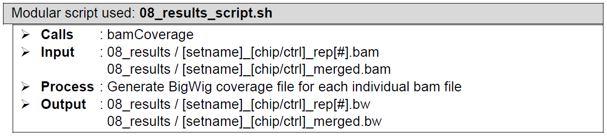
How does it look like? After 08_results_script.sh had been executed, the folder: 08_results will contain all these sorted reads files (marked by the extension: .bam), a couple merged sorted reads files* (marked by the extension: _merged.bam), indices to all the sorted reads files (marked by the extension: .bam.bai), the same sorted reads files re-sorted by name (marked by the extension: namesorted.bam), bigwig files of all the sorted reads files (marked by the extension: .bw), fingerprint plot files of all the sorted reads files (in its own folder: fingerprint_plots), and all the log files from all the program calls by 08_results_script.sh.
The left figure shows a single-end dataset with four ChIP samples and three control samples. The right figure shows a paired-end dataset with two ChIP samples and two control samples. There should be one sorted reads file here for each processed MAPQ-filtered reads file from folder 07_MAPQ_filtering; a merged ChIP and a merged control reads files*; one index file for each sorted reads file in this folder; one name-sorted reads file for each sorted reads file in this folder**; one bigwig file for each sorted reads file in this folder; two fingerprint plot files in the fingerprint_plots folder (in extension: .png and .svg); and another two fingerprint plot files in the fingerprint_plots folder (in extension: .png and .svg)***.
To view and analyze the read distribution of your peaks, load the BigWig files (.bw) into the program: IGV (more details down below). To view and evaluate your ChIP experiment DNA pulldown efficiency, open the .png or .svg using any supporting image viewer program (more details down below).
* Only when needed by the pipeline
** Except the merged ones
*** Only when merged sorted reads files are present -
Aligned reads quality assessment. Processed by FastQC. Quality assessment is performed to check for the alignment efficiency, such as how many reads failed to be mapped. Assessment results are saved as reports.
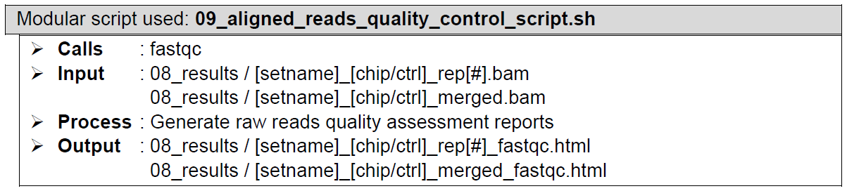
How does it look like? After 09_aligned_reads_quality_control_script.sh had been executed, the folder: 09_aligned_reads_quality_control will contain all these quality assessment reports for every .bam file in folder 08_results, just like below:
The left figure shows a single-end dataset with four ChIP samples and three control samples. The right figure shows a paired-end dataset with two ChIP samples and two control samples.
The .zip files contains the individual components to be compiled for the report so you can ignore those. To read the reports, open the .html files in your web-browser of choice (Safari, Edge, Firefox). This file is a multitabular file in which you can evaluate the quality of your experiment, sequencing, etc. Comprehensive as it is, explaining the contents in detail would take a whole new guide by itself. Therefore, its best to check out the documentation of the developers for all the details: https://www.bioinformatics.babraham.ac.uk/projects/fastqc/Help/.
-
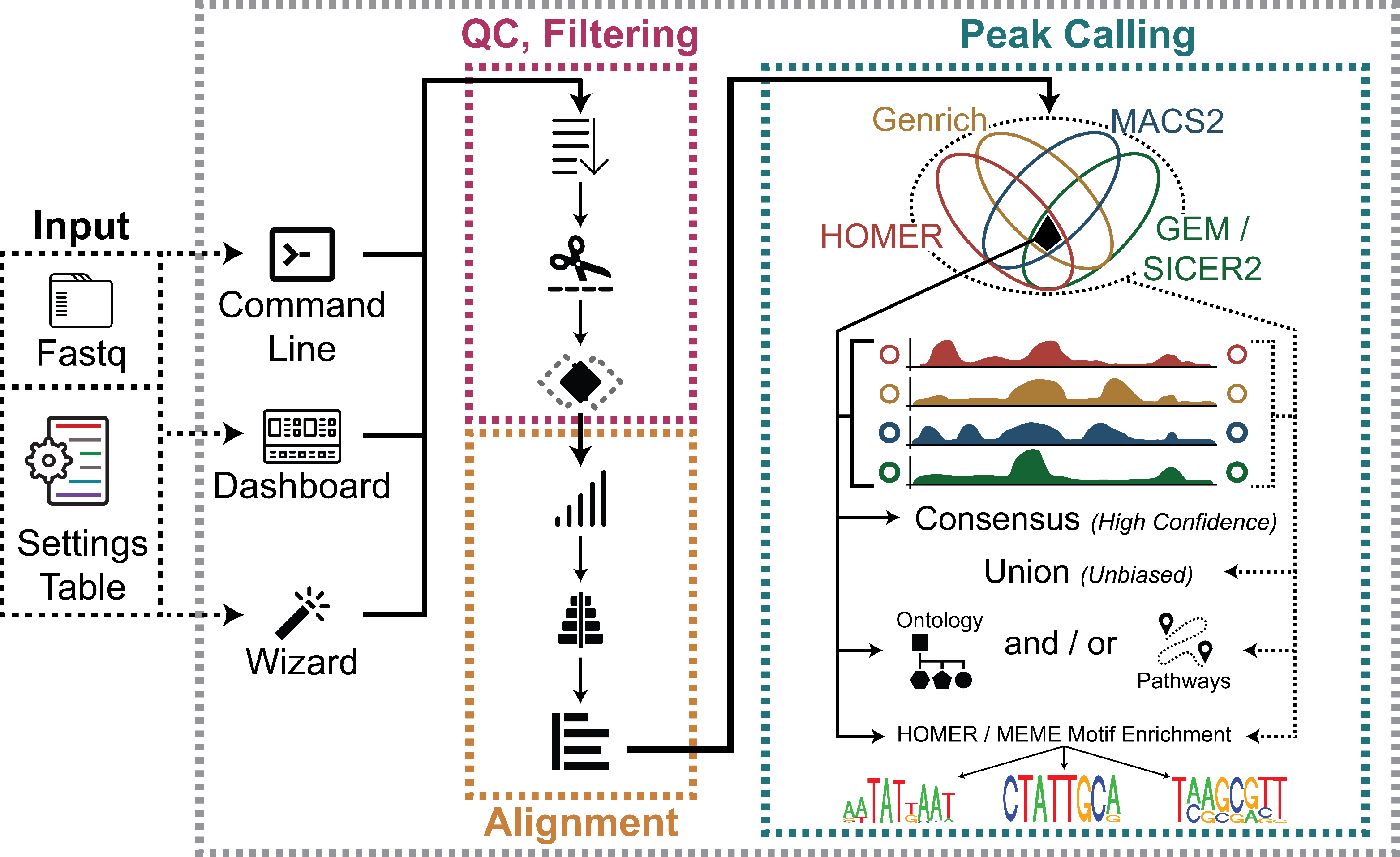
Peak calling. Multiple peak caller programs are involved in this step.
For Transcription Factors - Performed by MACS2 (default setting), GEM, HOMER (factor setting), and Genrich for transcription factor proteins of interest.
For Broad Peaks (Histone Marks) - Performed by MACS2 (broad setting), SICER2, HOMER (broad setting), and Genrich for histone modifier protein of interest.
The same track of aligned reads is scanned for potential protein-DNA binding sites.The process returns a list of enriched regions in various formats.MACS
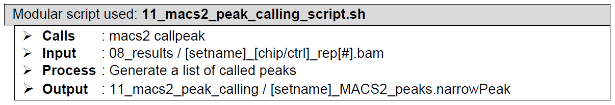
How does it look like? After 11_macs2_peak_calling_script.sh had been executed, the folder: 11_macs2_peak_calling will contain all these files, just like below:
For some reason, MACS2 does not generate the statistical model of the dataset’s background noise (.r) in paired-end mode (right figure).
MACS2 generates three output files, which all are basically peak lists, but each of these has their own exclusive information. In datasets with narrow peak type (left figure) the file that contains all necessary information relevant to analysis by ChIP-AP is the one with .narrowPeak extension. The peaks.xls file has the pileup value and peak length information, which tells us about the overall coverage of the corresponding peak region. The summits.bed basically are just lists of only the peak summits coordinates and read depth at the respective 1 base coordinate.
On the other hand, in datasets with broad peak type (right figure) the file that contains all necessary information relevant to analysis by ChIP-AP is the one with .broadPeak extension. The .gappedPeak file is basically a variant of .broadPeak, which is dedicated for peaks with both narrow and broad characteristics mixed in together, and thus has values that describes where and how deep are the “thick” and “thin” regions along each peak. As in the case of narrow peak type, the peaks.xls file has the pileup value and peak length information, which tells us about the overall coverage of the corresponding peak region. No summits.bed file generated in this case because of the absence of such “summit” in broad peaks.
The .narrowPeak file which ChIP-AP utilizes, has the following columns:
- chrom - Name of the chromosome (or contig, scaffold, etc.).
- chromStart - The starting position of the feature in the chromosome or scaffold. The first base in a chromosome is numbered 0.
- chromEnd - The ending position of the feature in the chromosome or scaffold. The chromEnd base is not included in the display of the feature. For example, the first 100 bases of a chromosome are defined as chromStart=0, chromEnd=100, and span the bases numbered 0-99.
- name - Name given to a region. Use "." if no name is assigned.
- score - Indicates how dark the peak will be displayed in the browser (0-1000). If all scores were "'0"' when the data were submitted to the DCC, the DCC assigned scores 1-1000 based on signal value. Ideally the average signalValue per base spread is between 100-1000.
- strand - +/- to denote strand or orientation (whenever applicable). Use "." if no orientation is assigned.
- signalValue - Overall (usually, average) enrichment for the region.
- pValue - Statistical significance (-log10). Use -1 if no pValue is assigned.
- qValue - Statistical significance using false discovery rate (-log10). Use -1 if no qValue is assigned.
- peak - Point-source called for this peak; 0-based offset from chromStart. Use -1 if no point-source called.
GEM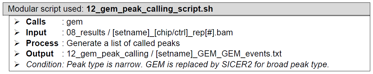
How does it look like? After 12_gem_peak_calling_script.sh had been executed, the folder: 12_gem_peak_calling will contain all these files, just like below:
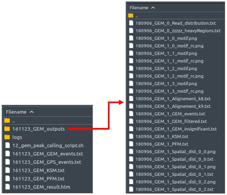
GEM outputs both the binding event files and the motif files. Because of the read distribution re-estimation, GEM outputs event prediction and read distribution files for multiple rounds. All of these are in saved in folder [setname]_GEM_outputs. However, as long as ChIP-AP is concerned, we are only interested in GEM’s final output files, which are saved outside the said folder. Each of these has their own exclusive information. GEM is actually a suite consisting of multiple modules performing their specific tasks. The GPS module is the one that detects peaks based on reads distribution (similar to most peak callers). The resulting peak list from solely running this GPS module can be viewed in file [setname]_GEM_GPS_events.txt.
However, GEM is also equipped with motif enrichment analysis module that helps improve true peaks detection. This GPS peak list is then processed further and modified based on the motif enrichment analysis, resulting in the final peak list in file [setname]_GEM_GEM_events.txt, which is the one utilized by ChIP-AP.
GEM also generates two secondary output files [setname]_GEM_KSM.txt and [setname]_GEM_PFM.txt, which are more of motif enrichment results rather than peak lists, and thus will not be discussed further here. Do check the GEM documentation link provided at the end of this guide if you are interested. Lastly, [setname]_GEM_result.htm is a web-based comprehensive summary of all the binding events and motifs.
The _GEM_events.txt file which ChIP-AP utilizes, has the following columns:
- Location - The genome coordinate of this binding event
- IP binding strength - The number of IP reads associated with the event
- Control binding strength - the number of control reads in the corresponding region
- Fold - Fold enrichment (IP/Control)
- Expected binding strength - The number of IP read counts expected in th binding region given its local context (defined by parameter W2 or W3), this is used as the Lambda parameter for the Poisson test
- Q_-lg10 - -log10(q-value), the q-value after multiple-testing correction, using the larger p-value of Binomial test and Poisson test
- P_-lg10 - -log10(p-value), the p-value is computed from the Binomial test given the IP and Control read counts (when there are control data)
- P_poiss - -log10(p-value), the p-value is computed from the Poisson test given the IP and Expected read counts (without considering control data)
- IPvsEMP - Shape deviation, the KL divergence of the IP reads from the empirical read distribution (log10(KL)), this is used to filter predicted events given the --sd cutoff (default=-0.40).
- Noise - The fraction of the event read count estimated to be noise
- KmerGroup - The group of the k-mers associated with this binding event, only the most significant k-mer is shown, the n/n values are the total number of sequence hits of the k-mer group in the positive and negative training sequences (by default total 5000 of each), respectively
- KG_hgp - log10(hypergeometric p-value), the significance of enrichment of this k-mer group in the positive vs negative training sequences (by default total 5000 of each), it is the hypergeometric p-value computed using the pos/neg hit counts and total counts
- Strand - The sequence strand that contains the k-mer group match, the orientation of the motif is determined during the GEM motif discovery, '*' represents that no k-mer is found to associated with this event
SICER2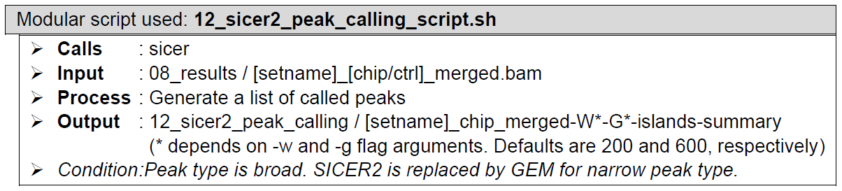
How does it look like? After 12_sicer2_peak_calling_script.sh had been executed, the folder: 12_sicer2_peak_calling will contain all these files, just like below:
SICER2 generates multiple output files as follows:
- [setname]_chip_merged-W*-G*-.scoreisland: delineation of significant islands controlled by E- value of 1000. It is in “chrom start end score” format.
- [setname]_chip_merged-W*-normalized.wig: wig file that can be used to visualize the windows generated by SICER2. Read count is normalized by library size per million.
- [setname]_chip_merged-W*-G*-islands-summary: summary of all candidate islands with their statistical significance. It is a tab-separated-values file that has the following columns format: chrom, start, end, ChIP_island_read_count, CONTROL_island_read_count, p_value, fold_change, FDR_threshold.
- [setname]_chip_merged-W*-G*-FDR*-island.bed: delineation of significant islands filtered by false discovery rate (FDR). It has the following format: chrom, start, end, read-count.
The file that contains all necessary information relevant to analysis by ChIP-AP is the one with [setname]_chip_merged-W*-G*-islands-summary.
HOMER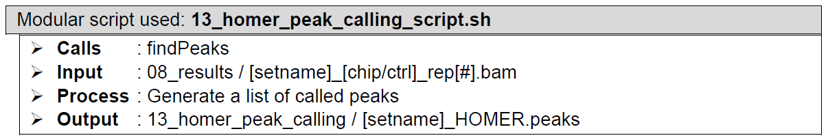
How does it look like? After 13_homer_peak_calling_script.sh had been executed, the folder: 13_homer_peak_calling will contain all these files, just like below:
There is no output files difference between single-end and paired-end mode.
Even though HOMER has different modes for narrow peak type (using flag argument -style factor) and broad peak type (using flag argument -style histone), the output files stay the same and so do the contents of these files, except for column 7 (see below).
The HOMER.peaks file which CHIP-AP utilizes, has the following columns:
- PeakID - Unique name for each peak
- chr - Chromosome where peak is located
- start - Starting position of peak
- end - Ending position of peak
- Strand (+/-)
- Normalized Tag Counts - Number of tags found at the peak, normalized to 10 million total mapped tags (or defined by the user)
- Focus Ratio - Fraction of tags found appropriately upstream and downstream of the peak center. (when sample peak type = narrow), OR Region Size - Length of enriched region (when sample peak type = broad)
- Peak score (read HOMER annotatePeaks documentation for details)
- Total Tags - Peak depth in the ChIP sample (normalized to control)
- Control Tags - Peak depth in the control sample
- Fold Change vs Control - Peak depth fold change of ChIP compared to control
- p-value vs Control - Statistical significance of ChIP peak compared to control
- Fold Change vs Local - Peak depth fold change of ChIP compared to its surrounding regions
- p-value vs Local - Statistical significance of ChIP peak compared to its surrounding regions
- Clonal Fold Change - Statistical significance of ChIP peak considering the abundance of read fragment clones, or duplicates
Genrich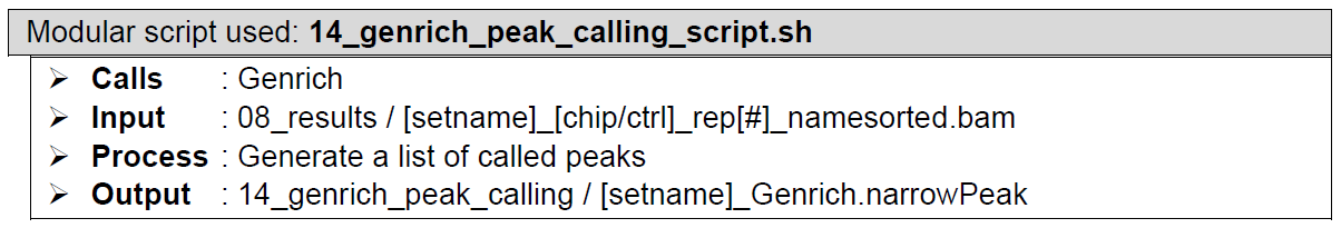
How does it look like? After 14_genrich_peak_calling_script.sh had executed, the folder: 14_genrich_peak_calling will contain all these files, just like below:
There is no output files difference between single-end and paired-end mode.
The .narrowPeak file which ChIP-AP utilizes, has the following columns:
- chrom - Name of the chromosome (or contig, scaffold, etc.).
- chromStart - The starting position of the feature in the chromosome or scaffold. The first base in a chromosome is numbered 0.
- chromEnd - The ending position of the feature in the chromosome or scaffold.The chromEnd base is not included in the display of the feature. For example, the first 100 bases of a chromosome are defined as chromStart=0, chromEnd=100, and span the bases numbered 0-99.
- name - Name given to a region. Use "." if no name is assigned.
- score - Indicates how dark the peak will be displayed in the browser (0-1000). If all scores were "'0"' when the data were submitted to the DCC, the DCC assigned scores 1-1000 based on signal value. Ideally the average signalValue per base spread is between 100-1000.
- strand - +/- to denote strand or orientation (whenever applicable). Use "." if no orientation is assigned.
- signalValue - Overall (usually, average) enrichment for the region.
- pValue - Statistical significance (-log10). Use -1 if no pValue is assigned.
- qValue - Statistical significance using false discovery rate (-log10). Use -1 if no qValue is assigned.
- peak - Point-source called for this peak; 0-based offset from chromStart. Use -1 if no point-source called.
-
Peaks merging. Performed by a custom script and HOMER’s mergePeaks. The custom script reformats necessary peak caller outputs into HOMER region list format. mergePeaks looks for overlaps between the regions in the four peak caller outputs and lists the merged regions in multiple files based on the peak caller(s) that calls them. These multiple files are then concatenated together into a single regions list file.
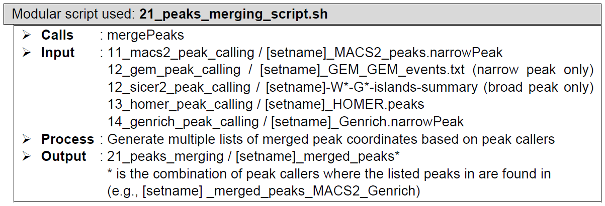
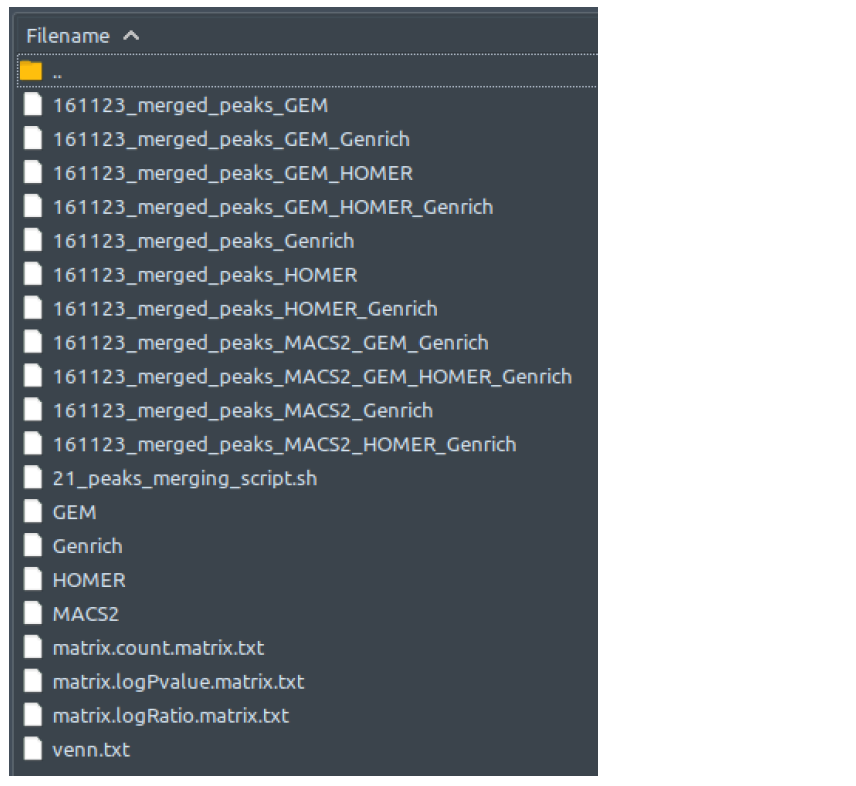
How does it look like? After 21_peaks_merging_script.sh had executed, the folder: 21_peaks_merging will contain all these files, just like below:
There is no output files difference between single-end and paired-end mode. Also, you will find SICER2 instead of GEM when running broad peak type datasets.
ChIP-AP takes the input files described above, then generates the four tab-separated-values files MACS2, GEM or SICER2, HOMER, and Genrich, which are lists of peaks detected by their respective peak caller.With MACS2, GEM or SICER2, HOMER, and Genrich as the input peak list, HOMER mergePeaks generates separate files based on overlapping peaks for each set of peaks: 21_peaks_merging/[setname]_merged_peaks*, where * is the combination of peak callers where the listed peaks in are found in. Files with certain peak callers combinations that contains zero peak will be non-existent in this folder, so don’t be alarmed if, for example, you cannot find [setname]_merged_peaks_MACS2_GEM file. That simply means that there is no peak that is detected ONLY by MACS2 and GEM, just like what we can see from the example above.
The following three matrix.txt files (below) are the secondary outputs of HOMER mergePeaks. These files contains the statistics about the pairwise overlap of peaks between the four callers peak sets, which could provide additional information for you despite them not being of any use for further processes down the line. The explanations below are taken directly from HOMER documentation - no further explanation is given by HOMER, so we cannot give a clearer explanation:
- matrix.logPvalue.matrix.txt: natural log p-values for overlap using the hypergeometric distribution, positive values signify divergence
- matrix.logRatio.matrix.txt: natural log of the ratio of observed overlapping peaks to the expected number of overlapping peaks
- matrix.count.matrix.txt: raw counts of overlapping peaks
Finally, there is the file venn.txt. This contains the numbers needed for you to create a Venn diagram depicting the peak overlaps between the four peak caller sets. Some custom scripts are available online which are able to directly take this venn.txt file as an input and generates a Venn diagram image as a result.
The resulting multiple 21_peaks_merging/[setname]_merged_peaks* files are then concatenated together into a single list file [setname]_all_peaks_concatenated.tsv by 22_peaks_processing_script.sh (the subsequent script in the pipeline), and saved in folder 22_peaks_processing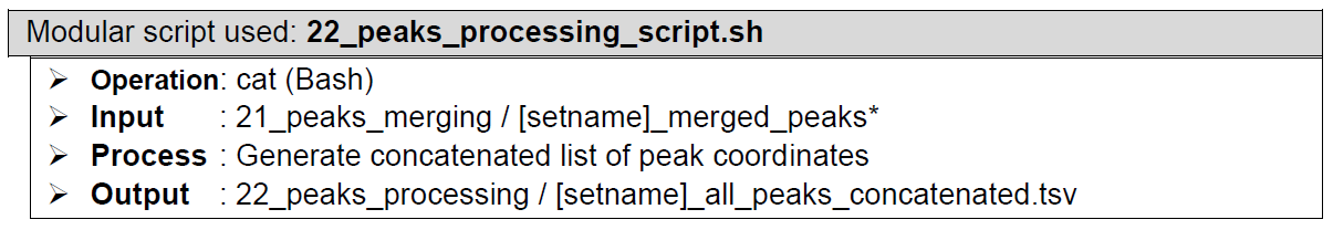
How does it look like? Detailed output preview of this step, step 18, 19, 20, and 21 are combined below step 21
-
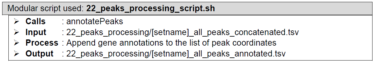
Peaks annotation. Performed by annotatePeaks from HOMER package. Each region in the concatenated list is annotated based on its genomic location for the genome specified. The process returns the same list of regions, with each entry row appended with various information pertaining to the gene name, database IDs, category, and instances of motif (if HOMER known motif matrix file is provided to ChIP-AP), etc.
How does it look like? Detailed output preview of step 18, 19, 20, and 21 are combined below step 21
-
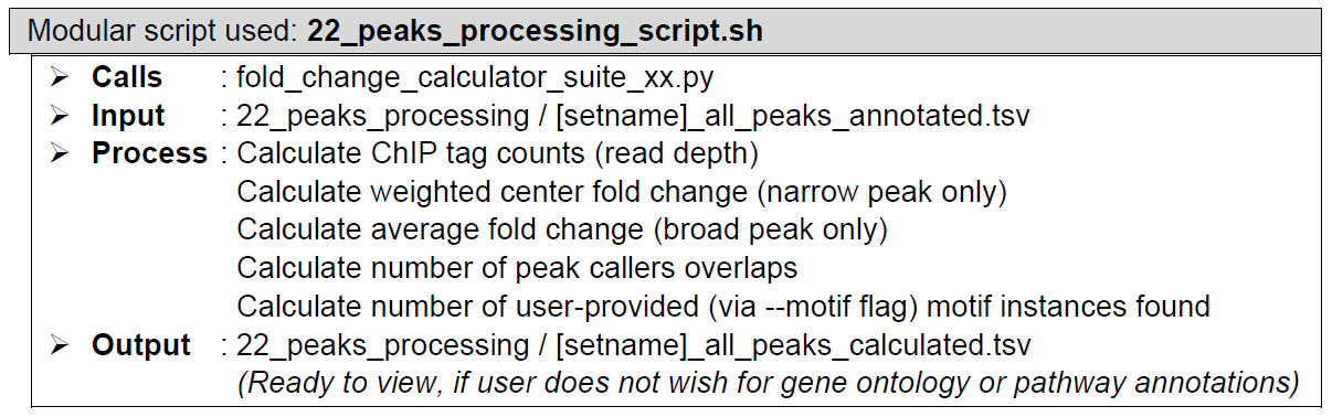
Fold enrichment calculations. Performed by a custom script, with the help of samtools depth and view modules. For weighted peak center fold enrichment calculations in cases of narrow peak type datasets, the custom script sends out the reformatted genomic regions as command line arguments for multi-threaded samtools depth runs. Samtools depth returns a list of read depths at each base within the region and saves them in a temporary file. The script then reads the temporary files and determine the weighted peak centers and returns the read depth values along with the base locations. The custom script sends out the weighted peak center base locations as command line arguments for multi-threaded samtools view runs. Samtools view returns the read depth values at the given base locations. The custom script then calculates the fold enrichment values, corrected based on the ChIP-to-control normalization factor.
For average fold enrichment calculation in cases of broad peak type datasets, samtools view simply sums up the number of reads in the whole peak region, then calculates the fold enrichment values, corrected based on the ChIP-to-control normalization factor.
In addition, the custom-made script also makes some reformatting and provides additional information necessary for downstream analysis.
How does it look like? Detailed output preview of step 18, 19, 20, and 21 are combined below step 21
-
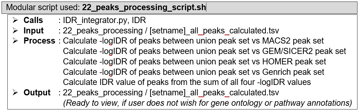
Irreproducibility rate (IDR) calculation. Performed by a custom script plugged to IDR module. The IDR module compares two different peak sets and assign to each listed peak in both peak sets an irreproducibility rate (IDR) value based on that peak’s capacity to be recalled by the other peak set. IDR value of each peak listed in the full (union) peak list ([setname]_all_peaks_calculated.tsv) was obtained by pairing it against every individual peak caller sets, followed by calculating the pair-wise -logIDR values, then summing them all up, and finally converting it into a final IDR value. The final IDR value shows the chance of a finding (i.e., the peak) being unable to be reproduced by different peak calling algorithms. This step reprocesses the peak list [setname]_all_peaks_calculated.tsv, augment the table with relevant IDR values, and re-save it under the same file name. For more details about IDR calculation method, see the IDR module documentations.
How does it look like? Detailed output preview of step 18, 19, 20, and 21 are combined below step 21
-
Peak statistics summary. Performed by a custom script designed for quality assessment of called peaks. Returns a summary text file containing information pertaining to the peak read depth, peak fold enrichment, known motif hits, and positive peak hits (based on known motif presence if a HOMER formatted motif file was included when calling ChIP-AP), in each peak set along the continuum between single peak callers and the absolute consensus of all four peak callers.
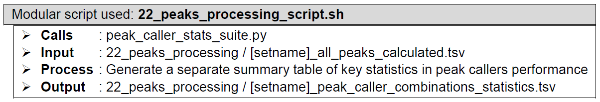
How does it look like? After 22_peaks_processing_script.sh had executed, the folder: 22_peaks_processing will contain all these files, just like below:
The last segment of step 17 concatenates all the peak caller combinations peak list files into one file: [setname]_all_peaks_concatenated.tsv, followed by annotation in step 18 that generates the file: [setname]_all_peaks_annotated.tsv, followed by fold change calculation etc. in step 19 that generates the file: [setname]_all_peaks_calculated.tsv. Step 20 reads the resulting file [setname]_all_peaks_calculated.tsv and generates a statistics summary file [setname]_peak_caller_combinations_statistics.tsv.
While HOMER annotatePeaks is working on annotating our concatenated peak list, it also performs a gene ontology enrichment analysis which generates several tab-separated-values text files as depicted in the right figure. Each of these files contains ranked list of enriched terms coming from specific genome ontology or pathway database. As ChIP-AP will only further append [setname]_peak_caller_combinations_statistics.tsv with terms from certain databases (optional; activated by "--goann" and/or "--pathann" flag), not all files generated here will be used further in the pipeline. The files used are biological_process.txt, molecular_function.txt, cellular_component.txt, interactions.txt, cosmic.txt, kegg.txt, biocyc.txt, pathwayInteractionDB.txt, reactome.txt, smpdb.txt, and wikipathways.txt.
The following three matrix.txt and a stats.txt files below are the secondary outputs of HOMER annotatePeaks. These files contain the statistics about the co-occurrence of motif instances (provided with "--motif" flag argument) in the peak sets, which could provide some additional information to you despite not being any use for further processes down the pipeline. These explanations below are taken directly from HOMER documentation - no further explanation is given by HOMER, so we cannot give a clearer explanation:
- setname.count.matrix.txt - number of peaks with motif co-occurrence
- setname.ratio.matrix.txt - ratio of observed vs. expected co-occurrence
- setname.logPvalue.matrix.txt - co-occurrence enrichment
- setname.stats.txt - table of pair-wise motif co-occurrence statistics
At this point, the results are actually ready to for your to view and analyze as they already have the essential information typically needed for ChIP-seq analysis. More details are described in the section below: Main Pipeline Output - Final Analysis Table. Here is a quick summary of what these are and why are they relevant to your analysis.
[setname]_all_peaks_concatenated.tsv already has information pertaining to:- Peak ID
- Chr
- Start
- End
- Strand
- Peak Caller Combination
So, if you basically only need to know where the peaks are, and which peak caller managed to detect particular peaks, this will suffice. For example: if you want to overlap the list detected peaks with your list of genomic coordinates (e.g., of genome-wide motif instance locations, or genome-wide histone marker locations, or regions of interests obtained from different experiment, or peak list you obtained by using your favorite peak caller etc.).
[setname]_all_peaks_annotated.tsv has these following information in addition to what is already in [setname]_all_peaks_concatenated.tsv:- Annotation
- Detailed Annotation
- Distance to TSS
- Nearest PromoterID
- Entrez ID
- Nearest Unigene
- Nearest Refseq
- Nearest Ensembl
- Gene Name
- Gene Alias
- Gene Description
- Gene Type
- CpG%
- GC%
At this point, the peak list is finally something biologically relevant, as each peak is now appended with the information that can be used to infer role and functionality at cellular or organism level, based on the nearest gene from the peak coordinate. As the protein used in ChIP pulldown experiments are typically transcription factor or histone modifier, a binding event in the close vicinity to a gene suggests regulation of gene expression. For instance, if you analyze this together with RNAseq differentially expressed genes data, then you might find which genes or which pathways your protein of interest is upregulating or downregulating.
As these peaks are now also equipped by the multiple databases’ ID of their nearest genes, the user can now connect this peak list with another list which entries are identified by a specific unique ID (e.g., ChIP-AP supplementary annotations relies on individual peak’s Entrez ID in order to connect to HOMER genome ontology database.
[setname]_all_peaks_calculated.tsv has these following information in addition to what is already in [setname]_all_peaks_annotated.tsv:- Peak Caller Overlaps
- ChIP Tag Count
- Control Tag Count
- Fold Change
- Number of Motifs
At this point, you have more power to evaluate and select the peaks you want in your final set. In this file you now have the actual read depth of your peaks, and also the fold change value where you can see the enrichment of reads at the potential binding site compared to the control sample with no pulldown. Along with that, each peak also have the number of known DNA binding motif found in the sample. Note that this value will only appear if you provided the .motif file using the "--motif" flag argument. These values provided here are the most basic properties of peaks pertaining to their confidence, and are the most standard ways of filtering and ranking of peaks in the list. These values are provided here as an alternative way to apply some thresholds in order to select your peak set for further analysis, in addition to the more powerful main method provided by this pipeline: multiple peak caller overlaps.
At this point, the peak list now has the number of peak caller overlaps, which is the number of peak callers that detected this peak. Although user can already filter in or out their peak list based on the peak caller names provided by the column “Peak Caller Combination” in the file [setname]_all_peaks_concatenated.tsv, this value is here to give user a more convenient way of filtering their peaks based on how many peak callers “agree” with a particular detected peak, regardless of which peak callers detected it.
-
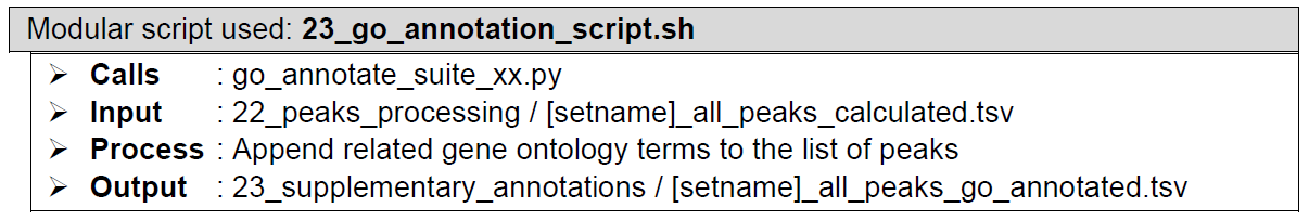
(Optional) Downstream analysis: Gene ontology enrichment. Each peak in the concatenated list is appended with all the gene ontology terms associated with its gene annotation. The gene ontology terms are derived from biological processes, molecular functions, and cellular compartments databases. This enables list filtering based on the gene ontology terms of the study’s interest.
-
(Optional) Downstream analysis: Pathway enrichment. Each peak in the concatenated list is appended with all the related biological pathways associated with its gene annotation. The biological pathway terms are derived from KEGG, SMPDB, Biocyc, Reactome, Wikipathways, and pathwayInteractionDB databases. This enables list filtering based on the biological pathways of the study’s interest. Additionally, this analysis also adds other terms pertaining to known interactions with common proteins and known gene mutations found in malignant cases, derived from common protein interaction and COSMIC databases, respectively.
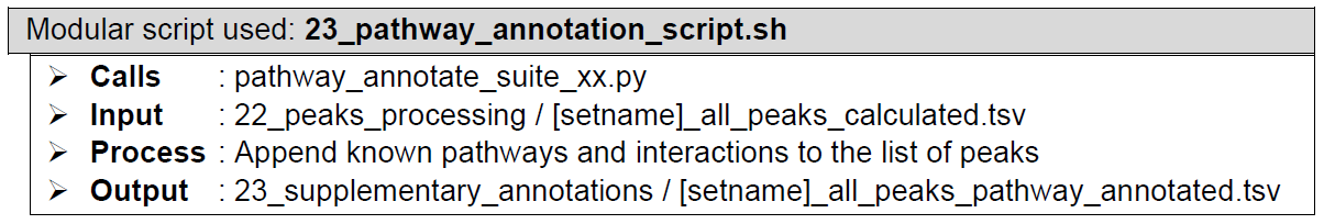
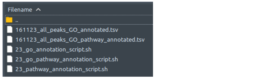
How does it look like? After 23_go_annotation_script.sh had executed, the folder: 23_supplementary_annotations will contain all these files, just like below:
There is no output files difference between single-end and paired-end mode.
If "--goann flag" is used during ChIP-AP call, 23_go_annotation_script.sh will be executed, and generates [setname]_all_peaks_go_annotated.tsv that contains the following gene ontology terms based on each peak’s nearest gene:
- Biological Process
- Molecular Function
- Cellular Component
If "--pathann" flag is used during ChIP-AP call, 23_pathway_annotation_script.sh will be executed, and generates [setname]_all_peaks_pathway_annotated.tsv that contains the following known pathways terms based on each peak’s nearest gene:
- Interaction with Common Protein
- Somatic Mutations (COSMIC)
- Pathway (KEGG)
- Pathway (BIOCYC)
- Pathway (pathwayInteractionDB)
If both "--goann" flag and "--pathann" flag are used during ChIP-AP call, both 23_go_annotation_script.sh and 23_pathway_annotation_script.sh will be executed, and generates [setname]_all_peaks_go_pathway_annotated.tsv that contains all the information that are gained by running the two scripts one after another:
- Biological Process
- Molecular Function
- Cellular Component
- Interaction with Common Protein
- Somatic Mutations (COSMIC)
- Pathway (KEGG)
- Pathway (BIOCYC)
- Pathway (pathwayInteractionDB)
These columns contains ALL the related terms from their respective gene ontology or pathway databases, which are comma-separated between terms. That said, depending on how developed the databases are, and how much is known about the gene, the amount of information can range between none to overwhelming.
The information is very useful for filtering the peak list based on the protein of interest’s potential roles in specific biological activities or pathways, based on the interest of the study. This can also be very handy, because contrary to the conventional way of only looking at the gene ontology enrichment analysis result and manually checking back-and-forth if specific genes of interest are actually related to specific terms of interest, we have it already linked to each peak in the list.
However, with respect to users who do not need such information and probably want their list to be much less verbose and smaller in size, this step is completely optional. The output files will not be generated, to save processing time should the user choose to omit this step (by not using the respective flags or not ticking the boxes in the GUI). The scripts will still be generated by ChIP-AP, though, just not executed. You can simply run the script should you change your mind and decide to have these supplementary annotations.
-
(Optional) Downstream analysis: Motif enrichment analysis with HOMER. Genomic sequences are extracted based on the coordinates of the peaks in consensus (four peak callers overlap), union (all called peaks), or both peak lists. HOMER performs analysis to identify specific DNA sequence motifs to which the experimented protein(s) have binding affinity towards. For the sake of processing speed, HOMER utilizes cumulative binomial distribution to calculate motif enrichment by default. However, by utilizing ChIP-AP custom setting table, user may choose to utilize cumulative hypergeometric distribution, which describes motif enrichment problem more accurately. Besides the typically performed calculations for de novo motifs discovery, HOMER also calculates the enrichment scores of the known motifs in HOMER motifs database. Since the relevance of protein-DNA binding events are mainly more restricted to the context of transcription factors compared to its histone modifiers counterpart, this optional downstream analysis option is only available for datasets with narrow (transcription factor) peaks.
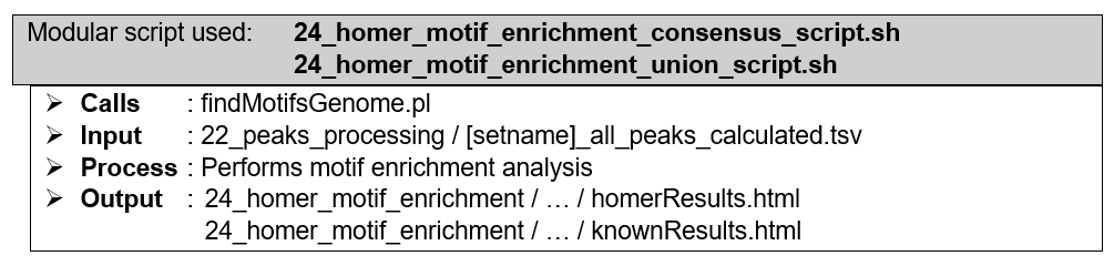
How does it look like? After 24_homer_motif_enrichment_consensus_script.sh or 24_homer_motif_enrichment_union_script.sh (or both scripts) had executed, the folder: 24_homer_motif_enrichment will contain these files, just like below:
If --homer_motif consensus flag and argument are used during ChIP-AP call, 24_homer_motif_enrichment_consensus_script.sh will be executed, and generates HOMER findMotifsGenome.pl output folders and files depicted by the image to the right, inside folder consensus_peak_set. If --homer_motif union flag and argument are used during ChIP-AP call, 24_homer_motif_enrichment_union_script.sh will be executed, and generates similar output inside folder union_peak_set. If --homer_motif both flag and argument are used during ChIP-AP call, both aforementioned scripts will be executed separately, generating output files and folders inside their respective folders.
-
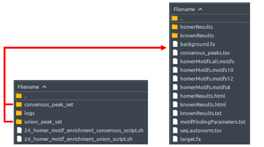
(Optional) Downstream analysis: Motif enrichment analysis with MEME. Genomic sequences are extracted based on the coordinates of the peaks in consensus (four peak callers overlap), union (all called peaks), or both peak lists. With or without control sequences extracted from random genomic sequences, MEME performs analysis to identify specific DNA sequence motifs to which the experimented protein(s) have binding affinity towards. By utilizing separate dedicated modules included in MEME suite, MEME-ChIP performs de novo motif discovery, motif enrichment analysis, motif location analysis and motif clustering in one go, providing a comprehensive picture of the DNA motifs that are enriched in the extracted sequences. MEME-ChIP performs two complementary types of de novo motif discovery: weight matrix–based discovery for high accuracy, and word-based discovery for high sensitivity. Since the relevance of protein-DNA binding events are mainly more restricted to the context of transcription factors compared to its histone modifiers counterpart, this optional downstream analysis option is only available for datasets with narrow (transcription factor) peaks.
How does it look like? After 25_meme_motif_enrichment_consensus_script sh or 25_meme_motif_enrichment_union_script.sh (or both scripts) had executed, the folder: 25_meme_motif_enrichment will contain these files, just like below:
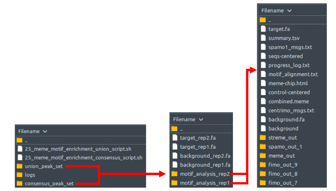
If --meme_motif consensus flag and argument are used during ChIP-AP call, 25_meme_motif_enrichment_consensus_script.sh will be executed, and generates meme-chip output folders and files depicted by the image in the middle, inside folder consensus_peak_set. If --meme_motif union flag and argument are used during ChIP-AP call, 25_meme_motif_enrichment_union_script.sh will be executed, and generates similar output inside folder union_peak_set. If --meme_motif both flag and argument are used during ChIP-AP call, both aforementioned scripts will be executed separately, generating output files and folders inside their respective folders.
When ChIP and control aligned reads (.bam) have the same number of replicates, ChIP-AP gives the option for merged (with --fcmerge flag) or pair-wise (without --fcmerge flag) fold change calculations. In pair-wise mode, peaks every ChIP vs control replicate have different weighted peak center coordinate, which directly affects the actual target and background sequences for meme-chip to perform enrichment analysis on. Therefore, ChIP-AP recognizes and processes multiple replicates separately (based on each weighted peak center coordinate), generating respective results for each replicate, stored in separate folders. On the contrary, whenever user choose to use --fcmerge flag, or when the number of ChIP and control samples are not the same, ChIP-AP will be forced to perform merged fold change calculation. In this situation every peak will have one weighted peak center coordinate and thus there will only be one replicate of meme-chip motif enrichment analysis results inside one single folder.
For most processes in every modular script, log files are recorded and saved in folder: /logs under their respective directories. There are two types of log files:
- Log files with .out extension: captures whatever the program writes out through channel 1>, a.k.a. the standard output
- Log files with .err extension: captures whatever the program writes out through channel 2>, a.k.a. the standard error
Sometimes, unlike what the file or channel name suggests, you might find errors reported in the .out files or something like normal program run progress report written in the .err files. That is just the way it is. Some programs do not follow the standard output / standard error convention, that’s why. So, if your pipeline crashed at a certain process and the .err log file does not show anything wrong, the error message might be in the .out file instead!
The example contents inside folder /logs can be seen below:
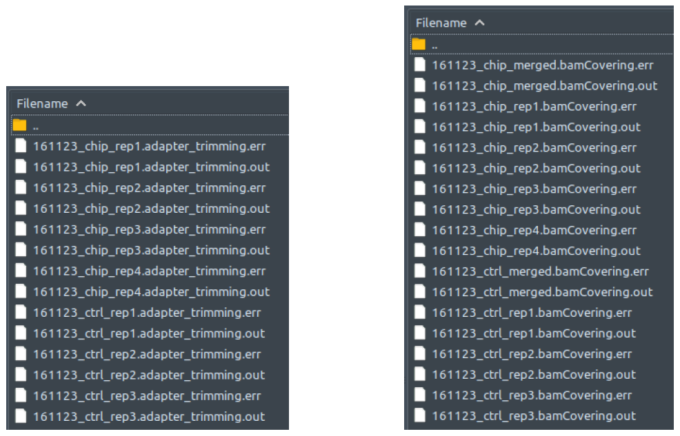
All these outputs are recorded for your convenience in troubleshooting and error reporting. Do open and read these files to see what’s happening with your program. After you spot the potential problem, you can either post the logged error message in our GitHub - issues (https://github.com/JSuryatenggara/ChIP-AP/issues), or go hit Google search if you think the problem is simple and quick enough to figure out yourself.
The table below shows the contents of [setname]_all_peaks_go_pathway_annotated.tsv. Smaller sized and less verbose variants of this table are saved in the output folder with suffixes: concatenated, annotated, and calculated (see Source in the table below)
| Column # | Peak Attribute | Source |
|---|---|---|
| Column 1 (A) | Peak ID (unique peak ID) |
Pipeline script: 22_peaks_ processing _script.sh Called program: cat (Bash) Output file: [setname]_all_peaks_concatenated.tsv Output folder: 22_peaks_processing |
| Column 2 (B) | Chr (chromosome) | |
| Column 3 (C) | Start (peak start coordinate) | |
| Column 4 (D) | End (peak end coordinate) | |
| Column 5 (E) | Strand (on which peak is found) | |
| Column 6 (F) | Peak Caller Combination | |
| Column 7 (G) | Peak Caller Overlaps |
Pipeline script: 22_peaks_processing_script.sh Called script: fold_change_calculator.py Output file: [setname]_all_peaks_calculated.tsv Output folder: 22_peaks_processing |
| Column 8 (H) | ChIP Tag Count | |
| Column 9 (I) | Control Tag Count | |
| Column 10 (J) | Fold Change | |
| Column 11 (K) | Peak Center | |
| Column 12 (L) | Number of Motifs | |
| Column 13 (M) | negLog10_IDR | |
| Column 14 (N) | IDR | |
| Column 15 (O) | Annotation |
Pipeline script: 22_peaks_processing_script.sh Called program: HOMER annotatePeaks Output file: [setname]_all_peaks_annotated.tsv Output folder: 22_peaks_processing |
| Column 16 (P) | Detailed Annotation | |
| Column 17 (Q) | Distance to TSS | |
| Column 18 (R) | Nearest PromoterID | |
| Column 19 (S) | Entrez ID | |
| Column 20 (T) | Nearest Unigene | |
| Column 21 (U) | Nearest Refseq | |
| Column 22 (V) | Nearest Ensembl | |
| Column 23 (W) | Gene Name | |
| Column 24 (X) | Gene Alias | |
| Column 25 (Y) | Gene Description | |
| Column 26 (Z) | Gene Type | |
| Column 27 (AA) | CpG% | |
| Column 28 (AB) | GC% | |
| Column 29 (AC) | Biological Process |
Pipeline script: 23_go_annotation_script.sh Called script: GO_annotator.py Output file: [setname]_all_peaks_go_annotated.tsv Output folder: 23_supplementary_annotations |
| Column 30 (AD) | Molecular Function | |
| Column 31 (AE) | Cellular Component | |
| Column 32 (AF) | Interaction with Common Protein |
Pipeline script: 23_pathway_annotation_script.sh Called script: pathway_annotator.py Output file: [setname]_all_peaks_pathway_annotated.tsv Output folder: 23_supplementary_annotations |
| Column 33 (AG) | Somatic Mutations (COSMIC) | |
| Column 34 (AH) | Pathway (KEGG) | |
| Column 35 (AI) | Pathway (BIOCYC) | |
| Column 36 (AJ) | Pathway (pathwayInteractionDB) | |
| Column 37 (AK) | Pathway (REACTOME) | |
| Column 38 (AL) | Pathway (SMPDB) | |
| Column 39 (AM) | Pathway (Wikipathways) |
| Peak Attribute | Description |
|---|---|
| Peak ID | Given unique peak ID |
| Chr | Chromosome where the peak is located |
| Start | Starting coordinate of the peak region |
| End | End coordinate of the peak region |
| Strand | DNA strand (positive/negative) where the peak is located |
| Peak Caller Combination | Name of peak callers that detected this peak |
| Peak Caller Overlaps | Number of peak callers that detected this peak |
| ChIP Tag Count | ChIP Read depth at weighted peak center (narrow peak) OR average read depth of the whole peak region (broad peak) |
| Control Tag Count | Control read depth at weighted peak center (narrow peak) OR average read depth of the whole peak region (broad peak) |
| Fold Change | ChIP vs control fold change at weighted peak center (narrow peak) OR ChIP vs control fold change of the whole peak region (broad peak) |
| Peak Center | Genomic coordinate of the weighted peak center (narrow peak) OR genomic coordinate of the of peak region midpoint (broad peak) |
| Number of Motifs | Number of motif instances found in the peak region |
| negLog10_IDR | Sum of - log10 IDR obtained from peak IDR calculation between the union and each individual peak caller set |
| IDR | Peak irreproducibility rate converted from negLog10_IDR column value |
| Annotation | Type of annotated region (Exon, Intron, Promoter-TSS) |
| Detailed Annotation | Detailed, longer version of Annotation in previous column |
| Distance to TSS | Distance from the peak to the nearest annotated Transcription Start Site (TSS) in basepairs |
| Nearest PromoterID | PromoterID of the nearest annotated promoter region |
| Entrez ID | Entrez ID of the nearest annotated gene |
| Nearest Unigene | Unigene ID of the nearest annotated gene |
| Nearest Refseq | Refseq ID of the nearest annotated gene |
| Nearest Ensembl | Ensembl ID of the nearest annotated gene |
| Gene Name | Name of the nearest annotated gene (abbreviated) |
| Gene Alias | Alternate names of the nearest annotated gene |
| Gene Description | Name of the nearest annotated gene (full) |
| Gene Type | e.g protein-coding / non-coding / pseudogene / etc |
| CpG% | The proportion of known methylation spots within this peak region |
| GC% | The proportion of GC contents within this peak region |
| Biological Process | Terms from biological_process.txt that are related to the nearest gene |
| Molecular Function | Terms from molecular_function.txt that are related to the nearest gene |
| Cellular Component | Terms from cellular component.txt that are related to the nearest gene |
| Interaction with Common Protein | Known interactions from interaction.txt with the nearest gene |
| Somatic Mutations (COSMIC) | Known cancer cases where mutation of the nearest gene are found |
| Pathway (KEGG) | Known pathways according to the KEGG database |
| Pathway (BIOCYC) | Known pathways according to the Biocyc database |
| Pathway (pathwayInteractionDB) | Known pathways from the pathwayInteractionDB database |
| Pathway (REACTOME) | Known pathways according to the REACTOME database |
| Pathway (SMPDB) | Known pathways according to the SMPDB database |
| Pathway (Wikipathways) | Known pathways according to the wikipathways database |
All the results are compiled and can be viewed by opening the file homerResults.html in an HTML file viewer such as your internet browser. This file gives you a formatted, organized view of the enriched de novo motifs and all the relevant information, as can be seen below. Additionally, more details can be accessed by simply clicking on the links in the table.
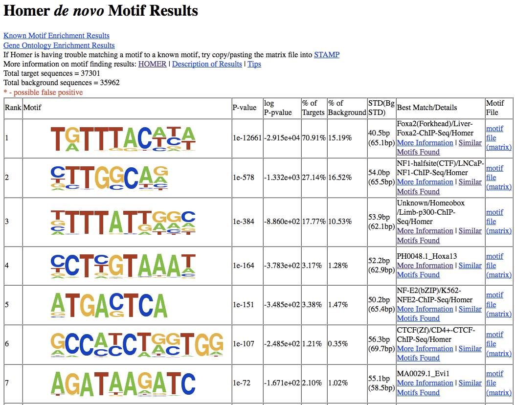
We can see these information listed below from the table:
| Column Name | Definition |
|---|---|
| Rank | Motif Rank |
| Motif | Motif position weight matrix logo |
| P-value | Final enrichment p-value |
| log P-pvalue | Log of p-value |
| % of Targets | Number of target sequences with motif/ total targets |
| % of Background | Number of background sequences with motif/ total background |
| STD(Bg STD) | Standard deviation of position in target and background sequences |
| Best Match/Details | Best match of de novo motif to motif database |
In addition to de novo motif enrichment, homer also performs motif enrichment analysis on the known binding motifs readily available within their database repertoire. The results for this analysis can be viewed in a similar way by opening the file knownResults.html, which contains similar information as its de novo counterpart.
More detailed information is available in http://homer.ucsd.edu/homer/ngs/peakMotifs.html
All the results are compiled and can be viewed by opening the file meme-chip.html in an HTML file viewer such as your internet browser. This file gives you a formatted, organized view of the enriched de novo motifs and all the relevant information. Additionally, more details can be accessed by simply clicking on the links in the table.
In datasets where there is an equal number of multiple-replicated ChIP and control samples, ChIP-AP will have MEME perform a pair-wise motif enrichment analysis. Therefore, in that case, there will be multiple replicates of motif enrichment results, each one looking like below.
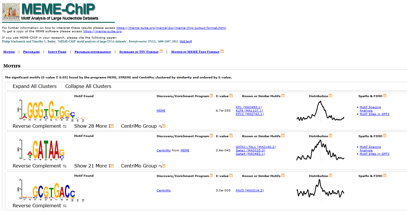
While the file above gives a more graphical representation of the results, meme-chip also generates another file: summary.tsv, which contains the same information (see below) repackaged in table format suitable for subsequent processing, if needed.
| Column Name | Definition |
|---|---|
| MOTIF_INDEX | The index of the motif in the "Motifs in MEME text format" file ('combined.meme') output by MEME-ChIP. |
| MOTIF_SOURCE | The name of the program that found the de novo motif, or the name of the motif file containing the known motif. |
| MOTIF_ID | The name of the motif, which is unique in the motif database file. |
| ALT_ID | An alternate name for the motif, which may be provided in the motif database file. |
| CONSENSUS | The ID of the de novo motif, or a consensus sequence computed from the letter frequencies in the known motif (as described below). |
| WIDTH | The width of the motif. |
| SITES | The number of sites reported by the de novo program, or the number of "Total Matches" reported by CentriMo. |
| E-VALUE | The statistical significance of the motif. |
| E-VALUE_SOURCE | The program that reported the E-value. |
| MOST_SIMILAR_MOTIF | The known motif most similar to this motif according to Tomtom. |
| URL | A link to a description of the most similar motif, or to the known motif. |
More detailed information is available in https://meme-suite.org/meme/doc/meme-chip.html
The table below shows the contents of [setname]_peak_caller_combinations_statistics.tsv.
| Column # | Peak Set Attribute |
|---|---|
| Column 1 (A) | Peak Callers Combination |
| Column 2 (B) | Exclusive Peak Count |
| Column 3 (C) | Exclusive Positive Peak Count |
| Column 4 (D) | Exclusive Motif Count |
| Column 5 (E) | Exclusive Positive Peak Hit Rate |
| Column 6 (F) | Exclusive Motif Hit Rate |
| Column 7 (G) | Exclusive ChIP Peak Read Depth |
| Column 8 (H) | Exclusive ChIP Peak Fold Change |
| Column 9 (I) | Inclusive Peak Count |
| Column 10 (J) | Inclusive Positive Peak Count |
| Column 11 (K) | Inclusive Motif Count |
| Column 12 (L) | Inclusive Positive Peak Hit Rate |
| Column 13 (M) | Inclusive Motif Hit Rate |
| Column 14 (N) | Inclusive ChIP Peak Read Depth |
| Column 15 (O) | Inclusive ChIP Peak Fold Change |
| Description: | |
|---|---|
| Peak Callers Combination | Name of peak callers that detected this peaks subset |
| Peak Count | Number of peaks |
| Positive Peak Count | Number of peaks containing known binding motif (--motif) |
| Motif Count | Total number of binding motif instances |
| Positive Peak Hit Rate | Positive Peak Count divided by Peak Count |
| Motif Hit Rate | Motif Count divided by Peak Count |
| ChIP Peak Read Depth | ChIP Read depth at weighted peak center (narrow peak) OR average read depth of the whole peak region (broad peak) |
| ChIP Peak Fold Change | ChIP vs control fold change in read depth |
-
Exclusive: Only counts for a specific peak caller combination (e.g., Exclusive peak count of MACS2 only counts for peaks that is exclusively called by MACS2 alone).
-
Inclusive: Counts for other peak caller combinations containing the same peak callers (e.g., Inclusive peak count of MACS2|GEM also counts for all other peaks in MACS2|GEM|HOMER, MACS2|GEM|Genrich, and MACS2|GEM|HOMER|Genrich).
This file summarizes the assignment of the files (IP sample or control, read 1 or 2; replicate number) and the file name conversion for every unaligned or aligned sequencing reads to be processed. Each line tells the user what the original files have been renamed into. Check this file if you suspect the order of samples were incorrectly entered (i.e., swapped chip with control)
Chromatin IP dataset replicate 1, 1st read : Original filename = a.fastq --> New filename = setname_chip_rep1_R1.fq.gz

Chromatin IP dataset replicate 2, 1st read : Original filename = b.fastq --> New filename = setname _chip_rep2_R1.fq.gz

Chromatin IP dataset replicate 1, 2nd read : Original filename = c.fastq --> New filename = setname _chip_rep1_R2.fq.gz

Chromatin IP dataset replicate 2, 2nd read : Original filename = d.fastq --> New filename = setname _chip_rep2_R2.fq.gz

Control dataset replicate 1, 1st read : Original filename = e.fastq --> New filename = setname _ctrl_rep1_R1.fq.gz

Control dataset replicate 2, 1st read : Original filename = f.fastq --> New filename = setname _ctrl_rep2_R1.fq.gz

Control dataset replicate 1, 2nd read : Original filename = g.fastq --> New filename = setname _ctrl_rep1_R2.fq.gz

Control dataset replicate 2, 2nd read : Original filename = h.fastq --> New filename = setname _ctrl_rep2_R2.fq.gz
Contains the input command line that was used to call the pipeline in a text file: [filename]_command_line.txt in the output save folder. This is useful for documentation of the run, and for re-running of the pipeline after a run failure or some tweaking if need be.
[chipap directory]/chipap.py --mode paired --ref [genome_build] --genome [path_to_computed_genome_folders] --output [full_path_to_output_save_folder] --setname [dataset name] --sample_table [path_to_sample_table_file] --custom_setting_table [path_to_setting_table_file].tsv --motif [path_to_known_motif_file] --fcmerge --goann --pathann --deltemp --thread [#_of_threads_to_use] --run
Contains the full path of each input ChIP and control sample in the pipeline run in a tab-separated value file: [setname]_sample_table.tsv in the output save folder in ChIP-AP sample table format. This is useful for documentation of the run, and for re-running of the pipeline after a run failure or some tweaking if need be. Below is an example of sample table file content (header included), given paired-end samples with two ChIP replicates and two control replicates:
| chip_read_1 | chip_read_2 | ctrl_read_1 | ctrl_read_2 |
|---|---|---|---|
| ... /a.fastq | ... /c.fastq | ... /e.fastq | ... /g.fastq |
| ... /b.fastq | ... /d.fastq | ... /f.fastq | ... /h.fastq |
If your sample is single-ended, then the '..._read_2' columns can be simple be left blank, or the sample table can be simplified to as follows:
| chip_read_1 | ctrl_read_1 |
|---|---|
| ... /a.fastq | ... /e.fastq |
| ... /b.fastq | ... /f.fastq |
A cornerstone of ChIP-AP’s functionality is the settings table. ChIP-AP, with the raw fq files and the settings table, is able to reproduce (near) identically any analysis that was performed (provided the same program version numbers are used). The ‘near identically’ statements is owing to the fact that reported alignments of multi-mappers may, in some cases, give every so slightly different results. This ambiguity can be alleviated however by filtering out alignments with low MAPQ scores in the corresponding alignment filter step, post-alignment to ensure consistent results from every analysis run. The provision of the settings table therefore ensures reproducibility of any analysis with minimal effort and bypasses the usually sparse and significantly under-detailed methods sections of publications. Science is supposed to be reproducible, yet bioinformatics analysis are typically black-boxes which are irreproducible. This 1 file, changes that!
The structure of the settings table is simple. It is a 2 column tab-separated value file with the names of the programs on the 1st column, and the necessary flags required or changed in the 2nd column. If making your own custom table, then the 1st column below must be copied as-is and not changed. These 2 columns together, list the flags and argument values for each program used in the pipeline.
When ChIP-AP is run, a copy of the used settings table is saved as a tab-separated value file: [setname]_ setting_table.tsv in the output save folder.
If you have a custom settings table made and provided it as input, then ChIP-AP will make a 2nd copy of this table in the same output save folder. This decision is made as it is useful documentation of the run performed. This file is also useful for re-running of the pipeline after run failure or some tweaking if necessary. If submitting an issue request on Github, you must provide us your settings table used as well as all other requested information. See Github for details regarding this.
We consider the dissemination of the information of this file as vital and essential along with results obtained. The table can be included as a supplemental table in a manuscript or can be included as a processed data file when submitting data to GEO – either way, the information of this file must be presented when publishing data.
Below is an example of setting table file in its default-setting state:
| program | argument |
|---|---|
| fastqc1 | -q |
| clumpify | dedupe spany addcount qout=33 fixjunk |
| bbduk | ktrim=r k=21 mink=8 hdist=2 hdist2=1 |
| trimmomatic | LEADING:20 SLIDINGWINDOW:4:20 TRAILING:20 MINLEN:20 |
| fastqc2 | -q |
| bwa_mem | |
| samtools_view | -q 20 |
| plotfingerprint | |
| fastqc3 | -q |
| macs2_callpeak | |
| gem | -Xmx10G --k_min 8 --k_max 12 |
| sicer2 | |
| homer_findPeaks | |
| genrich | --adjustp -v |
| homer_mergePeaks | |
| homer_annotatePeaks | |
| fold_change_calculator | --normfactor uniquely_mapped |
| homer_findMotifsGenome | -size given -mask |
| meme_chip | -meme-nmotifs 25 |
Ok so ChIP-AP does report a fair amount of stuff. If you ran it locally you have a swath of folders and you have nooooo clue what to look for and its all confusing. We get that. The reality though its very simple to know what to look for to know your experimental run worked and in this section were going to walk you through that!
There are a couple of things to look for to answer this question. 1, the fingerprint plot and 2, the venn diagram of the merged peaks. Let's begin…
-
The Fingerprint Plot
The fingerprint plot tells us how well the enrichment of your samples worked. It is generated by the function from the deeptools package and is generated after the alignment files. As such, the plots are found in the “08_results” folder and are labelled “fingerprint_xxxxx.png/svg.” The PNG files allow you to view them in any image viewer, the SVG files are for opening in Adobe Illustrator or Inkscape to make HQ publication figures later if you need.
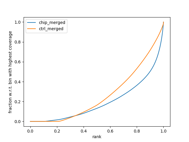
To interpret the fingerprint plot, (more information can be found on the deeptools documentation site), but put simply, the input control should be a diagonal line as close as possible toward the 1:1 diagonal. Your ChIP sample should have a bend/kink towards the bottom right corner. The greater the separation between the input and the chip sample, the greater the enrichment you will see in the final result (i.e., lots of peaks). If the lines are overlapping, then you will see little enrichment and your experiment didn’t work that well. If you’re sample lines are switched – then you probably switched the sample names and we recommend doing the right thing and repeating the experiment and not simply switch sample names for the sake of a publication.
In this example, there is reasonable enrichment in our chip samples. And so we are confident we can see enrichment.
-
The Venn Diagram (well Venn Text)
In the folder “21_peaks_merging” folder, you will find the “venn.txt” file. This will show you a textual venn diagram of the overlap between the called peaks across all peak callers. To know your experiment worked well, then you should see a full list with combinations of all peak callers and relatively large numbers for the consensus peak sets (ie peaks called by multiple peak callers) – this is the ideal case. However, from our experiences, there will almost always be 1 maybe 2 peak callers that don’t like a dataset for some reason and so you may find a peak caller performed poorly but the others performed admirably. This is still a good and valid result.
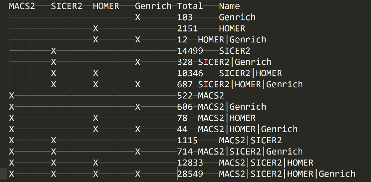
If you look at this file and only see a small number of peaks and little overlap, and only 1 peak caller seems to have dominated peak calling, then likely your experiment didn’t work that great. Just because only 1 peak caller performed well though, doesn’t mean the experiment is a write-off and a failure. It can still be valid and so doings some manual validations on the top FC differential peaks by chip-PCR might give you an indication whether there is salvageable data or not. Also if you have other confirmatory experimental evidence then even 1 peak calling getting results is fine. This is why we implemented multiple peak callers, because there are many instances where the signal:noise just creates a mess for most peak callers but generally 1 will be the super-hero of the day in such a situation.
-
What Results Files Do I Look At Exactly?
Valid question. In the folder “22_peak_processing,” open the “xxxx_all_peaks_calculated.tsv” file in excel and you’re good to go. Now to open it there is a little step to do…
Open a new blank workbook in excel

In the ribbon at the top, go to “Data”, then select “From Text/CSV”

In the dialog box that opens up, find and open the peaks files “xxxx_all_peaks_calculated.tsv.” Follow all the prompts and keep pressing “Next” / “Proceed” till the end and the file opens. Opening the peak file this way circumvents an issue that Excel constantly makes which is it will interpret some gene names such as OCT1 as a date, when its not. So by following the aforementioned steps, excel will not do this stupid conversion and instead, when you save the file as an xlsx, it will ensure that this issue doesn’t happen (seen it in sooooo many publications its not funny – just import data this way please people?)
From this file, you can view all the results and data for you analysis. Refer to Interpreting ChIP-AP Output for the definition of what each column means.
-
How Do I View My Alignments And Data?
People typically want to view their results on UCSC or other genome browsers. As we don’t have a web-server to host such coverage files (and making an accessible ucsc hub is a real pain and we don’t want to implement that), the onus is on you to view them locally on your machine. All laptops, whether then can run ChIP-AP or not can run IGV and view the coverage and bam files. The coverage and bam failes can be located in the “08_results” folder.
Download IGV, install it (super easy) and then load the coverage and bam files needed. Make sure you load the right genome build however! That’s critical. From the ChIP-AP main output file (see the Main Pipeline Output section), you can copy columns B,C,D straight into IGV and it will take you to the peak region.
-
In Short, What's Relevant?
Easy answers:-
Check fingerprint plot and make sure it looks good
-
Check venn.txt file and make sure you get good spread of peaks Together points 1 and 2 tell you your experiment worked!
-
Your final peak file is in “22_peak_processing” open the “xxxx_all_peaks_calculated.tsv” – This is the file you need to upload to GEO as your processed data file for your analysis and the only file you need to work with when looking through your data.
-
Also as part of your submission to GEO or as a supplemental table in your manuscript, you MUST include the settings table named “default_settings_table.txt” located in the root analysis directory. This provided with the raw fq files, which must be uploaded to GEO, will ensure complete reproducibility of the analysis performed.
-
Manuscript details for M&M. A statement such as the following should suffice:
For processing our ChIP-Seq analysis, we utilized ChIP-AP (https://academic.oup.com/bib/advance-article/doi/10.1093/bib/bbab537/6489109). Raw fq files are uploaded to GEO with accession number GSE172355, and the custom settings table utilized for analysis can be found on GEO as a processed settings file and also in Table 1 in our manuscript. Full details of ChIP-AP and its function can be found in its corresponding manuscript (https://academic.oup.com/bib/advance-article/doi/10.1093/bib/bbab537/6489109).
-
You can find all the details of every individual program through the links provided in the table below. Reading these is strongly recommended if you plan to modify ChIP-AP default settings.
Lastly, if you use ChIP-AP in your analysis, please cite us and all the following programs.