Welcome to the Finance-risk-analytics wiki!

Objective of analysis

The aim here, is to create an Indian credit risk(default) model, based on probability of default using logistic regression framework. We have an organization’s data with us, which is mainly categorized into 4 factors- Company's size, Profit, Leverage and Liquidity. We need to analyse our most significant features belong to these 4 factors, to find “Net-worth next year” - this represents the individual's company net worth for coming year. This is our dependent variable.

According to Sick Industrial Company Act (SICA, 1985), if a company is registered for more than 5 years and have incurred cash loss for two consecutive years, showing a negative net-worth is considered as sick company. They likely default. Here our dependent variable “Net-worth Next Year” will be marked as 1 when its value is negative, means the company will default. It will marked as 0 if the value remain positive, means the company will not default.

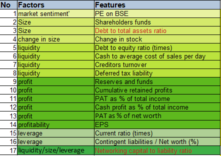
Features in our data set

The table above represents the features and its category, which information they describe.

We have total 52 variables describing features of the company or the balance sheet of an organisation. Total assets, income, capital, sales, net worth is present year represents a business size. Cost of equity at time of issue, changing stock price with market conditions, shares with the shareholders or with the company, capital employed after deducting all current liabilities from current assets gives information about the financial figure of the company owned by customer. Income from all sources, all reserves and funds, net profit after paying all taxes – these information help evaluating the annual profits made by the company. Negative figures indicates company is in loss.

Creditors turnovers, debtors turnovers, finished goods turnover, Raw material, WIP turnover informs the liquidity or cash available with the company in certain period of time. Cash from per day sales, cash with respect to current liabilities, shareholders funds gives a figure of cash availability at any point of time. Contingent liabilities gives figure of cash availability during uncertain events.

Only feature PE on BSE represents the market sentiment. It describes current stock price divided by its earning per share. Each feature in leverage category describes the money that is borrowed through various ways. Networking capital and total expenses are very important features which helps to know the expenses done by customer and net capital he has with them with respect to size of business.

Missing value treatment

Most of variables have missing values. As we have both positive and negative values in each variable so we are imputing the missing values with median. Except one variable, “Equity face value”. This variable has two value either 10 or 100 so to impute this I have used “MICE” technique.

Outliers

We have raw data set containing all information. “Num” and “Deposits accepted by all banks” are removed as they are observed non significant to model.
The above figure represents the outliers through multi variate analysis. Linear model of company data set where “net worth next year” is dependent variable and rest all are predictors. Cooks distance is used to find outliers and we have got only 8 outliers here. 8 out of 3541 observations, which very low than 3% of entire data set. So we are removing these outliers from data set.

New Variable creation

“Net worth next year” is converted to factor variable “Default...1”. 0 for positive net worth values and 1 for negative net worth values.
4 new variables are created with respect to leverage, liquidity, size and profit. Debt to total assets ratio is ratio obtained by dividing total “borrowings” and “total assets”. Debt to liability ratio is obtained by dividing total “borrowings” by “total liabilities”. Net working capital to liability ratio is obtained by dividing “net working capital” to “current liabilities”. PAT to asset ratio is obtained by dividing “Profit after tax” to “total asset”. Few of these variables are used in “altmaz Z score evaluation” for India.

Model creation

As we have many ratios and variables that are used to create those ratios in this data set, removing few of those primary variables to avoid multicollinearity issue. Below is the final set of variables used to create our linear regression model. Total 40 variables.

Balancing the data with SMOTE

We need a balanced data set to build logistic regression model as we have 93.37% non defaulters and 6.62% of defaulters. To bring balanced data set will use smote. The new data set “Balanced data” has both 50% defaulters and non defaulters.

Creating logistic regression model with most significant variables

In order to find the best variables to predicts defaulters we used “blr_step_aic_both() “ function from library “Blorr”. This function will do both forward selection and backward selection of variables from logmodel2 and provide us model with best AIC score. The above model displays the best model obtained from both forward and backward selection process. We are creating a new logistic regression model with those varibles of best model. This gives us an AIC score of 693.3. Now we have to do multicollinearity test to check if collinearity exists.
Multicollinearity test shows the “current time ratio” and “networking capital to liability ratio” has 10 and 11 respectively. So we have to remove one and rebuild the model.

Final model build with these features

ANALYSE COEFFICIENTS AND SIGNS

In our final model we have used total 16 variables. No multicollinearity is present, which confirms the vif test. From the Likelihood ratio test we have obtained a significant P-value, which means the Logistic regression model is valid.
The good news is in this model we all variables significant except “current time ratios”.This value too shows a significant odds ratio of 0.97 rest all variables are having odds ratio above this.

“Debt to equity ratio times" and “Debt to total asset ratio” turns out to be the most significant variables.
The values odds close to 0 indicates very low probability of default and odds value close to infinity shows very high probability of default. In logistic regression model increasing X by one unit changes the log odds by Beta 1.The amount of change in Y due to one unit change in X will depend on current value of X.
Positive sign : regardless of the value of X, if coefficient beta 1 is positive then increasing X will be associated with increasing Y.
Negative sign: if coefficient Beta 1 is negative then increasing X will be associated with decreasing Y.
Through maximum likelihood function we try to find coefficients beta1 beta2 such that plugging these estimates for Y , yields a number close to 1 for who has defaulted and number close to 0 who did not defaulted.
Debt to equity ratio Times: 0.3327,Debt to total asset ratio: 0.0193,Pat as of total income:0.003, contingent liabilities. Networth 0.003,cash to average cost of sales per day.

All these variables have Positive sign and coefficient value indicates that a unit increase in these variable values will increase the probability of default.
Shareholders funds: -0.0042, Reserves and funds, cumulative retained profits, EPS, change in stock, PE on BSE, PAT as of networth, deferred tax liabilities, cash profits as of total income, creditor turnovers, current ratio times- these variables have negative signs and coefficients value indicates that one unit increase in these values will decrease the probability of default.

PREDICT ACCURACY OF MODEL ON TRAIN AND VALIDATION DATASETS

Accuracy: Training model on the left shows accuracy of 85% and test model shows accuracy of 86%. 86% of the time it has predicted defaulters as defaulters and non-defaulters correctly.
Sensitivity: Training model sensitivity is 85% but test model sensitivity is 90%, which indicates its a better model. A customer who has defaulted if the model predicts it as non defaulters then, it will bring mode loss to financing parties.
Specificity: Training model specificity is 85% but test model specificity is also 85%. This predicts non_defaulters as defaulter. A false prediction but it does not create insecurities for financial companies but yes it is not good on company portfolio.

ROC CURVE

Ordering the customers

Our 10 deciles sorted in descending order and shows count of customers that will default or non default falls into each bucket.
So we have customer who probabilities of default is high and towards end probability of non_defaulters.
KS value is very low at the 10th decile and very high at the 1st decile which indicates the probability of defaulters are high in 1st bucket.

This is list of most significant variables which helps us predicting the customer who is going default or not default next year.
They belong to each of the 4 factors Size, leverage, liquidity and profit. Also our only variable in market sentiment turns out to be significant. Two ratios marked in RED are newly created variables from primary variables are also proved significant in predicting defaulters.