Programming Examples - ISET/isetcam GitHub Wiki
This page provides runnable code walkthroughs and links to rendered HTML tutorials generated with iePublish. The examples illustrate how code is structured and executed across three foundational tutorials:
-
t_introduction2ISET: A gentle, complete overview of the ISETCam computational flow. -
t_sceneIntroduction: In-depth exploration of thesceneobject, accessor methods (*Create,*Get,*Set,*Plot,*Window), parameter dependencies, and physical units. -
t_SystemSimulate: A comprehensive end-to-end camera simulation modeling optical blur, vignetting, Bayer pixel physics, sensor noise, and digital image processing.
- View Published HTML: t_introduction2ISET.html
-
Source Script:
tutorials/introduction/t_introduction2ISET.m
t_introduction2ISET introduces the core sequence of operations: creating a spectral radiance scene, modeling optical image formation, simulating sensor capture with calibrated color filters, and applying demosaicking and illuminant correction.
% Initialize the environment
ieInit;

% 1. Create a scene (Macbeth ColorChecker under tungsten light)
wave = 400:10:700;
scene = sceneCreate('macbeth tungsten', 64, wave);
scene = sceneAdjustIlluminant(scene, 'D65.mat'); % Change illuminant to D65
scene = sceneAdjustLuminance(scene, 200);        % Set mean luminance to 200 cd/m2
scene = sceneSet(scene, 'fov', 26.5);            % 26.5 deg field of view
sceneWindow(scene);

% 2. Calculate optical image irradiance using wavefront / diffraction optics
oi = oiCreate('wvf');
oi = oiSet(oi, 'optics fnumber', 2.8);
oi = oiSet(oi, 'optics offaxis method', 'cos4th');
oi = oiSet(oi, 'optics focal length', 3e-3);     % 3 mm focal length
oi = oiCompute(oi, scene);
oiWindow(oi);

% 3. Capture with a Bayer sensor
sensor = sensorCreate('bayer (rggb)');
sensor = sensorSet(sensor, 'auto exposure', true);
sensor = sensorCompute(sensor, oi);
sensorWindow(sensor);

% 4. Process sensor data into a display RGB image
ip = ipCreate;
ip = ipSet(ip, 'name', 'Color Balanced');
ip = ipSet(ip, 'internalCS', 'XYZ');
ip = ipSet(ip, 'conversion method sensor', 'MCC Optimized');
ip = ipSet(ip, 'correction method illuminant', 'Gray World');
ip = ipCompute(ip, sensor);
ipWindow(ip);- View Published HTML: t_sceneIntroduction.html
-
Source Script:
tutorials/scene/t_sceneIntroduction.m
t_sceneIntroduction demonstrates how to interact with ISETCam structures using *Create, *Get, *Set, *Plot, and *Window, and illustrates how dependent properties (like sample spacing) update automatically when primary parameters change.
ieInit;

% Create a Macbeth ColorChecker chart under D65 daylight
scene = sceneCreate('macbeth d65');
sceneWindow(scene);

% Get parameters
name = sceneGet(scene, 'name');          % 'Macbeth (D65)'
hFOV = sceneGet(scene, 'hfov');          % Horizontal field of view in degrees

% Set a parameter and observe dependent properties
scene = sceneSet(scene, 'hfov', 10);     % Change FOV to 10 degrees

% Query physical sample spacing in specified units
spacing_um = sceneGet(scene, 'sample spacing', 'um'); % In microns
spacing_mm = sceneGet(scene, 'sample spacing', 'mm'); % In millimeters

% Change distance: sample spacing updates automatically
scene = sceneSet(scene, 'distance', 1.2);             % Distance in meters
new_spacing_mm = sceneGet(scene, 'sample spacing', 'mm');

% Plot illuminant spectral power distribution in photons
scenePlot(scene, 'illuminant photons');

% Re-illuminate with a 5500 K blackbody radiator
bb = blackbody(sceneGet(scene, 'wave'), 5500, 'energy');
scene = sceneAdjustIlluminant(scene, bb);
sceneWindow(scene);

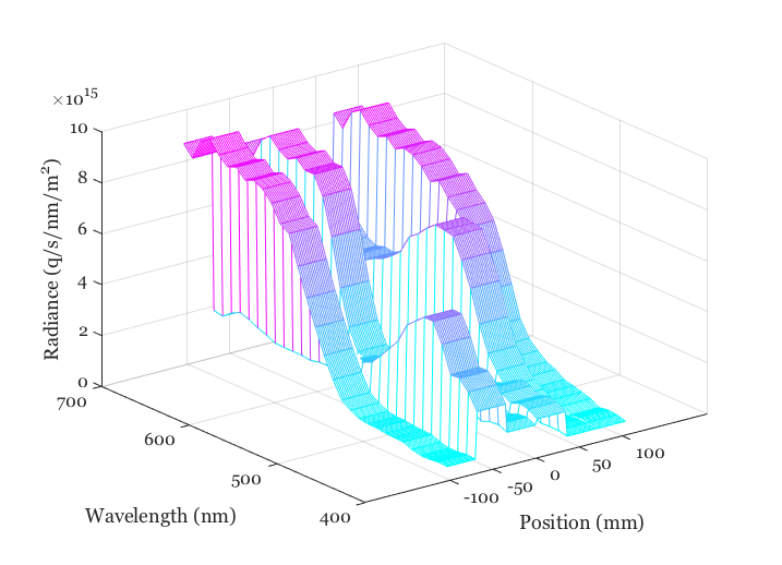
The Macbeth ColorChecker scene appearance (left) and 3D mesh plot of spectral radiance across spatial position and wavelength (right).
- View Published HTML: t_SystemSimulate.html
-
Source Script:
tutorials/camera/t_SystemSimulate.m
t_SystemSimulate details every component of the pipeline, configuring pixel well capacity, read noise, dark voltage, DSNU, PRNU, calibrated camera spectral quantum efficiencies (e.g., Nikon D100), and image processing pipelines.
ieInit;
wave = 400:10:700;

%% 1. Scene Creation
scene = sceneCreate('macbeth tungsten', 64, wave);
scene = sceneAdjustLuminance(scene, 100);  % 100 cd/m2 mean luminance
scene = sceneSet(scene, 'fov', 15);       % 15 deg field of view
sceneWindow(scene);

%% 2. Optical Image Formation
oi = oiCreate('diffraction');
oi = oiSet(oi, 'optics fnumber', 4);
oi = oiSet(oi, 'optics focal length', 3e-3);
oi = oiSet(oi, 'optics off axis method', 'cos4th');
oi = oiCompute(oi, scene);
oiWindow(oi);

%% 3. Sensor Capture & Noise Modeling
sensor = sensorCreate('bayer (gbrg)');

% Configure pixel geometry and noise
pixel = sensorGet(sensor, 'pixel');
pixel = pixelSet(pixel, 'size', [2.2e-6, 2.2e-6]);     % 2.2 um pixel size
pixel = pixelSet(pixel, 'voltageswing', 1.15);         % 1.15 V swing
pixel = pixelSet(pixel, 'conversiongain', 1.15 / 9000); % 9000 e- capacity
pixel = pixelSet(pixel, 'readnoisevolts', 0.00096);
sensor = sensorSet(sensor, 'pixel', pixel);

% Set sensor properties and noise levels
sensor = sensorSet(sensor, 'rows', 480);
sensor = sensorSet(sensor, 'cols', 640);
sensor = sensorSet(sensor, 'dsnu level', 0.0010);      % Dark signal non-uniformity
sensor = sensorSet(sensor, 'prnu level', 0.2218);      % Photo response non-uniformity
sensor = sensorSet(sensor, 'autoexposure', 1);

% Compute sensor voltages
sensor = sensorCompute(sensor, oi);
sensorWindow(sensor);

%% 4. Image Processing
ip = ipCreate;
ip = ipSet(ip, 'name', 'Color Balanced');
ip = ipSet(ip, 'internal cs', 'XYZ');
ip = ipSet(ip, 'conversion method sensor', 'MCC Optimized');
ip = ipSet(ip, 'illuminant correction method', 'Gray World');
ip = ipCompute(ip, sensor);
ipWindow(ip);

Scene spectral radiance (left) compared to the blurred and vignetted optical irradiance at the sensor plane (right).
-
Tutorials (
tutorials/t_*.m): Focused teaching scripts explaining core concepts. -
Examples (
examples/s_*.m): Applied workflow scripts and parameter sweeps designed to be adapted.
In the MATLAB Command Window, use tab completion to explore available files:
t_<TAB>       % Lists all tutorial scripts
s_<TAB>       % Lists all example scripts
s_scene<TAB>  % Lists example scripts for scenes
s_optics<TAB> % Lists example scripts for optics
s_sensor<TAB> % Lists example scripts for sensorsISETCam includes a publication engine based on MATLAB's publishing framework:
- The MATLAB script (
tutorials/.../t_*.m) is the executable source of truth. - Running
iePublish('tutorials/introduction/t_introduction2ISET.m')executes the script and embeds figures as inline base64 data within a standalone HTML file. - Batch scripts (
s_publishTutorials,s_publishExamples) regenerate HTML files acrosstutorials/andexamples/. - These rendered HTML files provide an interactive, illustrated counterpart to the code right from the wiki.