count_subset - HenrikBengtsson/matrixStats GitHub Wiki
matrixStats: Benchmark report
This report benchmark the performance of count() on subsetted computation.
> rvector <- function(n, mode = c("logical", "double", "integer"), range = c(-100, +100), na_prob = 0) {
+     mode <- match.arg(mode)
+     if (mode == "logical") {
+         x <- sample(c(FALSE, TRUE), size = n, replace = TRUE)
+     }     else {
+         x <- runif(n, min = range[1], max = range[2])
+     }
+     storage.mode(x) <- mode
+     if (na_prob > 0)
+         x[sample(n, size = na_prob * n)] <- NA
+     x
+ }
> rvectors <- function(scale = 10, seed = 1, ...) {
+     set.seed(seed)
+     data <- list()
+     data[[1]] <- rvector(n = scale * 100, ...)
+     data[[2]] <- rvector(n = scale * 1000, ...)
+     data[[3]] <- rvector(n = scale * 10000, ...)
+     data[[4]] <- rvector(n = scale * 1e+05, ...)
+     data[[5]] <- rvector(n = scale * 1e+06, ...)
+     names(data) <- sprintf("n = %d", sapply(data, FUN = length))
+     data
+ }
> data <- rvectors(mode = mode)> x <- data[["n = 1000"]]
> idxs <- sample.int(length(x), size = length(x) * 0.7)
> x_S <- x[idxs]
> gc()
used (Mb) gc trigger (Mb) max used (Mb)
Ncells 3230079 172.6 5709258 305.0 5709258 305.0
Vcells 12131425 92.6 28649958 218.6 56666022 432.4
> stats <- microbenchmark(count_x_S = count(x_S, value), `count(x, idxs)` = count(x, idxs = idxs, value),
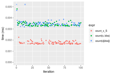
+ `count(x[idxs])` = count(x[idxs], value), unit = "ms")Table: Benchmarking of count_x_S(), count(x, idxs)() and count(x[idxs])() on integer+n = 1000 data. The top panel shows times in milliseconds and the bottom panel shows relative times.
| expr | min | lq | mean | median | uq | max | |
|---|---|---|---|---|---|---|---|
| 1 | count_x_S | 0.001619 | 0.0016630 | 0.0017513 | 0.0017065 | 0.0018110 | 0.002255 |
| 2 | count(x, idxs) | 0.003229 | 0.0033065 | 0.0034167 | 0.0033545 | 0.0034935 | 0.004806 |
| 3 | count(x[idxs]) | 0.003190 | 0.0033525 | 0.0049716 | 0.0034385 | 0.0035520 | 0.144710 |
| expr | min | lq | mean | median | uq | max | |
|---|---|---|---|---|---|---|---|
| 1 | count_x_S | 1.000000 | 1.000000 | 1.000000 | 1.000000 | 1.000000 | 1.000000 |
| 2 | count(x, idxs) | 1.994441 | 1.988274 | 1.950957 | 1.965719 | 1.929045 | 2.131264 |
| 3 | count(x[idxs]) | 1.970352 | 2.015935 | 2.838766 | 2.014943 | 1.961347 | 64.172949 |
Figure: Benchmarking of count_x_S(), count(x, idxs)() and count(x[idxs])() on integer+n = 1000 data. Outliers are displayed as crosses. Times are in milliseconds.
> x <- data[["n = 10000"]]
> idxs <- sample.int(length(x), size = length(x) * 0.7)
> x_S <- x[idxs]
> gc()
used (Mb) gc trigger (Mb) max used (Mb)
Ncells 3228239 172.5 5709258 305.0 5709258 305.0
Vcells 11802269 90.1 28649958 218.6 56666022 432.4
> stats <- microbenchmark(count_x_S = count(x_S, value), `count(x, idxs)` = count(x, idxs = idxs, value),
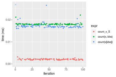
+ `count(x[idxs])` = count(x[idxs], value), unit = "ms")Table: Benchmarking of count_x_S(), count(x, idxs)() and count(x[idxs])() on integer+n = 10000 data. The top panel shows times in milliseconds and the bottom panel shows relative times.
| expr | min | lq | mean | median | uq | max | |
|---|---|---|---|---|---|---|---|
| 1 | count_x_S | 0.001666 | 0.0018615 | 0.0020140 | 0.0020160 | 0.0021335 | 0.003167 |
| 3 | count(x[idxs]) | 0.013703 | 0.0141310 | 0.0149449 | 0.0142755 | 0.0144655 | 0.060614 |
| 2 | count(x, idxs) | 0.016783 | 0.0170145 | 0.0172585 | 0.0171785 | 0.0173070 | 0.019913 |
| expr | min | lq | mean | median | uq | max | |
|---|---|---|---|---|---|---|---|
| 1 | count_x_S | 1.00000 | 1.000000 | 1.000000 | 1.000000 | 1.000000 | 1.000000 |
| 3 | count(x[idxs]) | 8.22509 | 7.591190 | 7.420595 | 7.081101 | 6.780173 | 19.139249 |
| 2 | count(x, idxs) | 10.07383 | 9.140209 | 8.569340 | 8.521081 | 8.112023 | 6.287654 |
Figure: Benchmarking of count_x_S(), count(x, idxs)() and count(x[idxs])() on integer+n = 10000 data. Outliers are displayed as crosses. Times are in milliseconds.

> x <- data[["n = 100000"]]
> idxs <- sample.int(length(x), size = length(x) * 0.7)
> x_S <- x[idxs]
> gc()
used (Mb) gc trigger (Mb) max used (Mb)
Ncells 3228311 172.5 5709258 305.0 5709258 305.0
Vcells 11865829 90.6 28649958 218.6 56666022 432.4
> stats <- microbenchmark(count_x_S = count(x_S, value), `count(x, idxs)` = count(x, idxs = idxs, value),
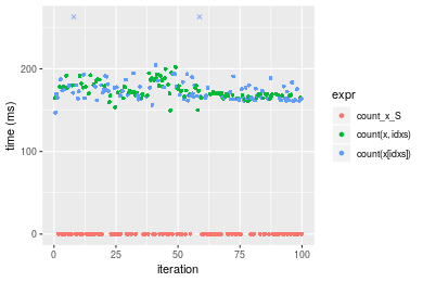
+ `count(x[idxs])` = count(x[idxs], value), unit = "ms")Table: Benchmarking of count_x_S(), count(x, idxs)() and count(x[idxs])() on integer+n = 100000 data. The top panel shows times in milliseconds and the bottom panel shows relative times.
| expr | min | lq | mean | median | uq | max | |
|---|---|---|---|---|---|---|---|
| 1 | count_x_S | 0.001643 | 0.0019185 | 0.0021756 | 0.0020645 | 0.0024935 | 0.002985 |
| 3 | count(x[idxs]) | 0.148818 | 0.1503995 | 0.1547928 | 0.1530510 | 0.1536240 | 0.268071 |
| 2 | count(x, idxs) | 0.190942 | 0.1922220 | 0.1966419 | 0.1965080 | 0.1970690 | 0.235942 |
| expr | min | lq | mean | median | uq | max | |
|---|---|---|---|---|---|---|---|
| 1 | count_x_S | 1.00000 | 1.00000 | 1.00000 | 1.00000 | 1.00000 | 1.00000 |
| 3 | count(x[idxs]) | 90.57699 | 78.39432 | 71.14786 | 74.13466 | 61.60979 | 89.80603 |
| 2 | count(x, idxs) | 116.21546 | 100.19390 | 90.38305 | 95.18431 | 79.03309 | 79.04255 |
Figure: Benchmarking of count_x_S(), count(x, idxs)() and count(x[idxs])() on integer+n = 100000 data. Outliers are displayed as crosses. Times are in milliseconds.

> x <- data[["n = 1000000"]]
> idxs <- sample.int(length(x), size = length(x) * 0.7)
> x_S <- x[idxs]
> gc()
           used  (Mb) gc trigger  (Mb) max used  (Mb)
Ncells  3228383 172.5    5709258 305.0  5709258 305.0
Vcells 12495878  95.4   28649958 218.6 56666022 432.4
> stats <- microbenchmark(count_x_S = count(x_S, value), `count(x, idxs)` = count(x, idxs = idxs, value),
+     `count(x[idxs])` = count(x[idxs], value), unit = "ms")
Table: Benchmarking of count_x_S(), count(x, idxs)() and count(x[idxs])() on integer+n = 1000000 data. The top panel shows times in milliseconds and the bottom panel shows relative times.
| expr | min | lq | mean | median | uq | max | |
|---|---|---|---|---|---|---|---|
| 1 | count_x_S | 0.001678 | 0.0021955 | 0.0073567 | 0.0049855 | 0.0125475 | 0.044432 |
| 2 | count(x, idxs) | 2.262734 | 2.3477680 | 2.5927281 | 2.4185615 | 2.7107550 | 5.827718 |
| 3 | count(x[idxs]) | 2.925195 | 3.0648270 | 3.5152259 | 3.1479515 | 3.5457175 | 14.266352 |
| expr | min | lq | mean | median | uq | max | |
|---|---|---|---|---|---|---|---|
| 1 | count_x_S | 1.000 | 1.000 | 1.0000 | 1.0000 | 1.0000 | 1.0000 |
| 2 | count(x, idxs) | 1348.471 | 1069.355 | 352.4299 | 485.1191 | 216.0395 | 131.1604 |
| 3 | count(x[idxs]) | 1743.263 | 1395.959 | 477.8252 | 631.4214 | 282.5836 | 321.0828 |
Figure: Benchmarking of count_x_S(), count(x, idxs)() and count(x[idxs])() on integer+n = 1000000 data. Outliers are displayed as crosses. Times are in milliseconds.

> x <- data[["n = 10000000"]]
> idxs <- sample.int(length(x), size = length(x) * 0.7)
> x_S <- x[idxs]
> gc()
           used  (Mb) gc trigger (Mb) max used  (Mb)
Ncells  3228455 172.5    5709258  305  5709258 305.0
Vcells 18795926 143.5   34459949  263 56666022 432.4
> stats <- microbenchmark(count_x_S = count(x_S, value), `count(x, idxs)` = count(x, idxs = idxs, value),
+     `count(x[idxs])` = count(x[idxs], value), unit = "ms")
Table: Benchmarking of count_x_S(), count(x, idxs)() and count(x[idxs])() on integer+n = 10000000 data. The top panel shows times in milliseconds and the bottom panel shows relative times.
| expr | min | lq | mean | median | uq | max | |
|---|---|---|---|---|---|---|---|
| 1 | count_x_S | 0.003185 | 0.006837 | 0.0213222 | 0.0111545 | 0.036879 | 0.067999 |
| 3 | count(x[idxs]) | 119.062488 | 132.784881 | 139.6765763 | 135.0524170 | 141.274531 | 392.878951 |
| 2 | count(x, idxs) | 118.899762 | 150.948282 | 151.9656970 | 152.2712185 | 154.161277 | 159.782806 |
| expr | min | lq | mean | median | uq | max | |
|---|---|---|---|---|---|---|---|
| 1 | count_x_S | 1.00 | 1.00 | 1.000 | 1.00 | 1.000 | 1.000 |
| 3 | count(x[idxs]) | 37382.26 | 19421.51 | 6550.752 | 12107.44 | 3830.758 | 5777.717 |
| 2 | count(x, idxs) | 37331.17 | 22078.15 | 7127.105 | 13651.10 | 4180.191 | 2349.782 |
Figure: Benchmarking of count_x_S(), count(x, idxs)() and count(x[idxs])() on integer+n = 10000000 data. Outliers are displayed as crosses. Times are in milliseconds.

> rvector <- function(n, mode = c("logical", "double", "integer"), range = c(-100, +100), na_prob = 0) {
+     mode <- match.arg(mode)
+     if (mode == "logical") {
+         x <- sample(c(FALSE, TRUE), size = n, replace = TRUE)
+     }     else {
+         x <- runif(n, min = range[1], max = range[2])
+     }
+     storage.mode(x) <- mode
+     if (na_prob > 0)
+         x[sample(n, size = na_prob * n)] <- NA
+     x
+ }
> rvectors <- function(scale = 10, seed = 1, ...) {
+     set.seed(seed)
+     data <- list()
+     data[[1]] <- rvector(n = scale * 100, ...)
+     data[[2]] <- rvector(n = scale * 1000, ...)
+     data[[3]] <- rvector(n = scale * 10000, ...)
+     data[[4]] <- rvector(n = scale * 1e+05, ...)
+     data[[5]] <- rvector(n = scale * 1e+06, ...)
+     names(data) <- sprintf("n = %d", sapply(data, FUN = length))
+     data
+ }
> data <- rvectors(mode = mode)> x <- data[["n = 1000"]]
> idxs <- sample.int(length(x), size = length(x) * 0.7)
> x_S <- x[idxs]
> gc()
used (Mb) gc trigger (Mb) max used (Mb)
Ncells 3228533 172.5 5709258 305 5709258 305.0
Vcells 17353131 132.4 34459949 263 56666022 432.4
> stats <- microbenchmark(count_x_S = count(x_S, value), `count(x, idxs)` = count(x, idxs = idxs, value),
+ `count(x[idxs])` = count(x[idxs], value), unit = "ms")Table: Benchmarking of count_x_S(), count(x, idxs)() and count(x[idxs])() on double+n = 1000 data. The top panel shows times in milliseconds and the bottom panel shows relative times.
| expr | min | lq | mean | median | uq | max | |
|---|---|---|---|---|---|---|---|
| 1 | count_x_S | 0.001658 | 0.0017330 | 0.0018447 | 0.001779 | 0.0019170 | 0.002773 |
| 2 | count(x, idxs) | 0.003308 | 0.0033625 | 0.0035267 | 0.003414 | 0.0035550 | 0.006260 |
| 3 | count(x[idxs]) | 0.003438 | 0.0036185 | 0.0042375 | 0.003720 | 0.0038325 | 0.048690 |
| expr | min | lq | mean | median | uq | max | |
|---|---|---|---|---|---|---|---|
| 1 | count_x_S | 1.000000 | 1.000000 | 1.000000 | 1.000000 | 1.000000 | 1.000000 |
| 2 | count(x, idxs) | 1.995175 | 1.940277 | 1.911854 | 1.919056 | 1.854460 | 2.257483 |
| 3 | count(x[idxs]) | 2.073583 | 2.087998 | 2.297137 | 2.091062 | 1.999218 | 17.558601 |
Figure: Benchmarking of count_x_S(), count(x, idxs)() and count(x[idxs])() on double+n = 1000 data. Outliers are displayed as crosses. Times are in milliseconds.

> x <- data[["n = 10000"]]
> idxs <- sample.int(length(x), size = length(x) * 0.7)
> x_S <- x[idxs]
> gc()
           used  (Mb) gc trigger (Mb) max used  (Mb)
Ncells  3228599 172.5    5709258  305  5709258 305.0
Vcells 17362618 132.5   34459949  263 56666022 432.4
> stats <- microbenchmark(count_x_S = count(x_S, value), `count(x, idxs)` = count(x, idxs = idxs, value),
+     `count(x[idxs])` = count(x[idxs], value), unit = "ms")
Table: Benchmarking of count_x_S(), count(x, idxs)() and count(x[idxs])() on double+n = 10000 data. The top panel shows times in milliseconds and the bottom panel shows relative times.
| expr | min | lq | mean | median | uq | max | |
|---|---|---|---|---|---|---|---|
| 1 | count_x_S | 0.001675 | 0.0019025 | 0.0020680 | 0.0020680 | 0.0022010 | 0.003167 |
| 3 | count(x[idxs]) | 0.016112 | 0.0167550 | 0.0178118 | 0.0170035 | 0.0173945 | 0.072023 |
| 2 | count(x, idxs) | 0.017637 | 0.0178775 | 0.0180867 | 0.0180085 | 0.0181525 | 0.022179 |
| expr | min | lq | mean | median | uq | max | |
|---|---|---|---|---|---|---|---|
| 1 | count_x_S | 1.000000 | 1.000000 | 1.000000 | 1.000000 | 1.000000 | 1.000000 |
| 3 | count(x[idxs]) | 9.619105 | 8.806833 | 8.613154 | 8.222195 | 7.902999 | 22.741711 |
| 2 | count(x, idxs) | 10.529552 | 9.396846 | 8.746090 | 8.708172 | 8.247388 | 7.003158 |
Figure: Benchmarking of count_x_S(), count(x, idxs)() and count(x[idxs])() on double+n = 10000 data. Outliers are displayed as crosses. Times are in milliseconds.
> x <- data[["n = 100000"]]
> idxs <- sample.int(length(x), size = length(x) * 0.7)
> x_S <- x[idxs]
> gc()
           used  (Mb) gc trigger (Mb) max used  (Mb)
Ncells  3228671 172.5    5709258  305  5709258 305.0
Vcells 17457495 133.2   34459949  263 56666022 432.4
> stats <- microbenchmark(count_x_S = count(x_S, value), `count(x, idxs)` = count(x, idxs = idxs, value),
+     `count(x[idxs])` = count(x[idxs], value), unit = "ms")
Table: Benchmarking of count_x_S(), count(x, idxs)() and count(x[idxs])() on double+n = 100000 data. The top panel shows times in milliseconds and the bottom panel shows relative times.
| expr | min | lq | mean | median | uq | max | |
|---|---|---|---|---|---|---|---|
| 1 | count_x_S | 0.001662 | 0.0019560 | 0.0022419 | 0.002221 | 0.0025330 | 0.002890 |
| 3 | count(x[idxs]) | 0.187506 | 0.1892825 | 0.2515486 | 0.196456 | 0.3197070 | 0.392828 |
| 2 | count(x, idxs) | 0.217537 | 0.2179915 | 0.2202523 | 0.218266 | 0.2186345 | 0.267948 |
| expr | min | lq | mean | median | uq | max | |
|---|---|---|---|---|---|---|---|
| 1 | count_x_S | 1.0000 | 1.00000 | 1.00000 | 1.00000 | 1.00000 | 1.00000 |
| 3 | count(x[idxs]) | 112.8195 | 96.77019 | 112.20481 | 88.45385 | 126.21674 | 135.92664 |
| 2 | count(x, idxs) | 130.8887 | 111.44760 | 98.24492 | 98.27375 | 86.31445 | 92.71557 |
Figure: Benchmarking of count_x_S(), count(x, idxs)() and count(x[idxs])() on double+n = 100000 data. Outliers are displayed as crosses. Times are in milliseconds.

> x <- data[["n = 1000000"]]
> idxs <- sample.int(length(x), size = length(x) * 0.7)
> x_S <- x[idxs]
> gc()
           used  (Mb) gc trigger (Mb) max used  (Mb)
Ncells  3228743 172.5    5709258  305  5709258 305.0
Vcells 18402936 140.5   34459949  263 56666022 432.4
> stats <- microbenchmark(count_x_S = count(x_S, value), `count(x, idxs)` = count(x, idxs = idxs, value),
+     `count(x[idxs])` = count(x[idxs], value), unit = "ms")
Table: Benchmarking of count_x_S(), count(x, idxs)() and count(x[idxs])() on double+n = 1000000 data. The top panel shows times in milliseconds and the bottom panel shows relative times.
| expr | min | lq | mean | median | uq | max | |
|---|---|---|---|---|---|---|---|
| 1 | count_x_S | 0.003542 | 0.0043465 | 0.013231 | 0.008344 | 0.0220045 | 0.035122 |
| 2 | count(x, idxs) | 7.223669 | 9.0095400 | 10.220966 | 9.615808 | 9.9312620 | 23.321479 |
| 3 | count(x[idxs]) | 5.099413 | 9.4980355 | 10.540235 | 10.415299 | 10.7106510 | 23.115483 |
| expr | min | lq | mean | median | uq | max | |
|---|---|---|---|---|---|---|---|
| 1 | count_x_S | 1.000 | 1.000 | 1.0000 | 1.000 | 1.0000 | 1.0000 |
| 2 | count(x, idxs) | 2039.432 | 2072.826 | 772.5020 | 1152.422 | 451.3287 | 664.0134 |
| 3 | count(x[idxs]) | 1439.699 | 2185.215 | 796.6324 | 1248.238 | 486.7482 | 658.1483 |
Figure: Benchmarking of count_x_S(), count(x, idxs)() and count(x[idxs])() on double+n = 1000000 data. Outliers are displayed as crosses. Times are in milliseconds.

> x <- data[["n = 10000000"]]
> idxs <- sample.int(length(x), size = length(x) * 0.7)
> x_S <- x[idxs]
> gc()
           used  (Mb) gc trigger  (Mb) max used  (Mb)
Ncells  3228812 172.5    5709258 305.0  5709258 305.0
Vcells 27852979 212.6   41431938 316.2 56666022 432.4
> stats <- microbenchmark(count_x_S = count(x_S, value), `count(x, idxs)` = count(x, idxs = idxs, value),
+     `count(x[idxs])` = count(x[idxs], value), unit = "ms")
Table: Benchmarking of count_x_S(), count(x, idxs)() and count(x[idxs])() on double+n = 10000000 data. The top panel shows times in milliseconds and the bottom panel shows relative times.
| expr | min | lq | mean | median | uq | max | |
|---|---|---|---|---|---|---|---|
| 1 | count_x_S | 0.004525 | 0.0070435 | 0.0224937 | 0.011471 | 0.041713 | 0.053685 |
| 3 | count(x[idxs]) | 147.007862 | 164.1726900 | 177.7612231 | 169.873675 | 178.636941 | 456.497123 |
| 2 | count(x, idxs) | 149.775005 | 167.5224960 | 174.0146670 | 170.718605 | 179.378404 | 201.964168 |
| expr | min | lq | mean | median | uq | max | |
|---|---|---|---|---|---|---|---|
| 1 | count_x_S | 1.00 | 1.00 | 1.000 | 1.00 | 1.000 | 1.000 |
| 3 | count(x[idxs]) | 32487.93 | 23308.40 | 7902.726 | 14808.97 | 4282.524 | 8503.253 |
| 2 | count(x, idxs) | 33099.45 | 23783.98 | 7736.165 | 14882.63 | 4300.300 | 3762.022 |
Figure: Benchmarking of count_x_S(), count(x, idxs)() and count(x[idxs])() on double+n = 10000000 data. Outliers are displayed as crosses. Times are in milliseconds.
R version 3.6.1 Patched (2019-08-27 r77078)
Platform: x86_64-pc-linux-gnu (64-bit)
Running under: Ubuntu 18.04.3 LTS

Matrix products: default
BLAS:   /home/hb/software/R-devel/R-3-6-branch/lib/R/lib/libRblas.so
LAPACK: /home/hb/software/R-devel/R-3-6-branch/lib/R/lib/libRlapack.so

locale:
 [1] LC_CTYPE=en_US.UTF-8       LC_NUMERIC=C
 [3] LC_TIME=en_US.UTF-8        LC_COLLATE=en_US.UTF-8
 [5] LC_MONETARY=en_US.UTF-8    LC_MESSAGES=en_US.UTF-8
 [7] LC_PAPER=en_US.UTF-8       LC_NAME=C
 [9] LC_ADDRESS=C               LC_TELEPHONE=C
[11] LC_MEASUREMENT=en_US.UTF-8 LC_IDENTIFICATION=C

attached base packages:
[1] stats     graphics  grDevices utils     datasets  methods   base

other attached packages:
[1] microbenchmark_1.4-6    matrixStats_0.55.0-9000 ggplot2_3.2.1
[4] knitr_1.24              R.devices_2.16.0        R.utils_2.9.0
[7] R.oo_1.22.0             R.methodsS3_1.7.1       history_0.0.0-9002

loaded via a namespace (and not attached):
 [1] Biobase_2.45.0       bit64_0.9-7          splines_3.6.1
 [4] network_1.15         assertthat_0.2.1     highr_0.8
 [7] stats4_3.6.1         blob_1.2.0           robustbase_0.93-5
[10] pillar_1.4.2         RSQLite_2.1.2        backports_1.1.4
[13] lattice_0.20-38      glue_1.3.1           digest_0.6.20
[16] colorspace_1.4-1     sandwich_2.5-1       Matrix_1.2-17
[19] XML_3.98-1.20        lpSolve_5.6.13.3     pkgconfig_2.0.2
[22] genefilter_1.66.0    purrr_0.3.2          ergm_3.10.4
[25] xtable_1.8-4         mvtnorm_1.0-11       scales_1.0.0
[28] tibble_2.1.3         annotate_1.62.0      IRanges_2.18.2
[31] TH.data_1.0-10       withr_2.1.2          BiocGenerics_0.30.0
[34] lazyeval_0.2.2       mime_0.7             survival_2.44-1.1
[37] magrittr_1.5         crayon_1.3.4         statnet.common_4.3.0
[40] memoise_1.1.0        laeken_0.5.0         R.cache_0.13.0
[43] MASS_7.3-51.4        R.rsp_0.43.1         tools_3.6.1
[46] multcomp_1.4-10      S4Vectors_0.22.1     trust_0.1-7
[49] munsell_0.5.0        AnnotationDbi_1.46.1 compiler_3.6.1
[52] rlang_0.4.0          grid_3.6.1           RCurl_1.95-4.12
[55] cwhmisc_6.6          rappdirs_0.3.1       labeling_0.3
[58] bitops_1.0-6         base64enc_0.1-3      boot_1.3-23
[61] gtable_0.3.0         codetools_0.2-16     DBI_1.0.0
[64] markdown_1.1         R6_2.4.0             zoo_1.8-6
[67] dplyr_0.8.3          bit_1.1-14           zeallot_0.1.0
[70] parallel_3.6.1       Rcpp_1.0.2           vctrs_0.2.0
[73] DEoptimR_1.0-8       tidyselect_0.2.5     xfun_0.9
[76] coda_0.19-3
Total processing time was 1.34 mins.
To reproduce this report, do:
html <- matrixStats:::benchmark('count_subset')Copyright Dongcan Jiang. Last updated on 2019-09-10 20:57:36 (-0700 UTC). Powered by RSP.
<script> var link = document.createElement('link'); link.rel = 'icon'; link.href = "data:image/png;base64,iVBORw0KGgoAAAANSUhEUgAAACAAAAAgCAMAAABEpIrGAAAA21BMVEUAAAAAAP8AAP8AAP8AAP8AAP8AAP8AAP8AAP8AAP8AAP8AAP8AAP8AAP8AAP8AAP8AAP8AAP8AAP8AAP8AAP8AAP8AAP8AAP8AAP8AAP8AAP8AAP8AAP8AAP8AAP8AAP8AAP8AAP8AAP8AAP8AAP8AAP8AAP8AAP8AAP8AAP8BAf4CAv0DA/wdHeIeHuEfH+AgIN8hId4lJdomJtknJ9g+PsE/P8BAQL9yco10dIt1dYp3d4h4eIeVlWqWlmmXl2iYmGeZmWabm2Tn5xjo6Bfp6Rb39wj4+Af//wA2M9hbAAAASXRSTlMAAQIJCgsMJSYnKD4/QGRlZmhpamtsbautrrCxuru8y8zN5ebn6Pn6+///////////////////////////////////////////LsUNcQAAAS9JREFUOI29k21XgkAQhVcFytdSMqMETU26UVqGmpaiFbL//xc1cAhhwVNf6n5i5z67M2dmYOyfJZUqlVLhkKucG7cgmUZTybDz6g0iDeq51PUr37Ds2cy2/C9NeES5puDjxuUk1xnToZsg8pfA3avHQ3lLIi7iWRrkv/OYtkScxBIMgDee0ALoyxHQBJ68JLCjOtQIMIANF7QG9G9fNnHvisCHBVMKgSJgiz7nE+AoBKrAPA3MgepvgR9TSCasrCKH0eB1wBGBFdCO+nAGjMVGPcQb5bd6mQRegN6+1axOs9nGfYcCtfi4NQosdtH7dB+txFIpXQqN1p9B/asRHToyS0jRgpV7nk4nwcq1BJ+x3Gl/v7S9Wmpp/aGquum7w3ZDyrADFYrl8vHBH+ev9AUASW1dmU4h4wAAAABJRU5ErkJggg==" document.getElementsByTagName('head')[0].appendChild(link); </script>