colRowOrderStats - HenrikBengtsson/matrixStats GitHub Wiki
matrixStats: Benchmark report
This report benchmark the performance of colOrderStats() and rowOrderStats() against alternative methods.
- apply() + quantile(..., type = 3L)
- Biobase::rowQ()
> rmatrix <- function(nrow, ncol, mode = c("logical", "double", "integer", "index"), range = c(-100,
+     +100), na_prob = 0) {
+     mode <- match.arg(mode)
+     n <- nrow * ncol
+     if (mode == "logical") {
+         x <- sample(c(FALSE, TRUE), size = n, replace = TRUE)
+     }     else if (mode == "index") {
+         x <- seq_len(n)
+         mode <- "integer"
+     }     else {
+         x <- runif(n, min = range[1], max = range[2])
+     }
+     storage.mode(x) <- mode
+     if (na_prob > 0)
+         x[sample(n, size = na_prob * n)] <- NA
+     dim(x) <- c(nrow, ncol)
+     x
+ }
> rmatrices <- function(scale = 10, seed = 1, ...) {
+     set.seed(seed)
+     data <- list()
+     data[[1]] <- rmatrix(nrow = scale * 1, ncol = scale * 1, ...)
+     data[[2]] <- rmatrix(nrow = scale * 10, ncol = scale * 10, ...)
+     data[[3]] <- rmatrix(nrow = scale * 100, ncol = scale * 1, ...)
+     data[[4]] <- t(data[[3]])
+     data[[5]] <- rmatrix(nrow = scale * 10, ncol = scale * 100, ...)
+     data[[6]] <- t(data[[5]])
+     names(data) <- sapply(data, FUN = function(x) paste(dim(x), collapse = "x"))
+     data
+ }
> data <- rmatrices(mode = mode)> X <- data[["10x10"]]
> gc()
used (Mb) gc trigger (Mb) max used (Mb)
Ncells 3164817 169.1 5709258 305.0 5709258 305.0
Vcells 6247177 47.7 22267496 169.9 56666022 432.4
> probs <- 0.3
> which <- round(probs * nrow(X))
> colStats <- microbenchmark(colOrderStats = colOrderStats(X, which = which, na.rm = FALSE), `apply+quantile` = apply(X,
+ MARGIN = 2L, FUN = quantile, probs = probs, na.rm = FALSE, type = 3L), `rowQ(t(X))` = rowQ(t(X),
+ which = which), unit = "ms")
> X <- t(X)
> gc()
used (Mb) gc trigger (Mb) max used (Mb)
Ncells 3162930 169.0 5709258 305.0 5709258 305.0
Vcells 6241821 47.7 22267496 169.9 56666022 432.4
> rowStats <- microbenchmark(rowOrderStats = rowOrderStats(X, which = which, na.rm = FALSE), `apply+quantile` = apply(X,
+ MARGIN = 1L, FUN = quantile, probs = probs, na.rm = FALSE, type = 3L), rowQ = rowQ(X, which = which),
+ unit = "ms")Table: Benchmarking of colOrderStats(), apply+quantile() and rowQ(t(X))() on integer+10x10 data. The top panel shows times in milliseconds and the bottom panel shows relative times.
| expr | min | lq | mean | median | uq | max | |
|---|---|---|---|---|---|---|---|
| 1 | colOrderStats | 0.001932 | 0.0031710 | 0.0049054 | 0.005677 | 0.0060760 | 0.018188 |
| 3 | rowQ(t(X)) | 0.014249 | 0.0182860 | 0.0231091 | 0.022621 | 0.0257695 | 0.108739 |
| 2 | apply+quantile | 0.700427 | 0.7188305 | 0.7642608 | 0.733271 | 0.7637415 | 1.015273 |
| expr | min | lq | mean | median | uq | max | |
|---|---|---|---|---|---|---|---|
| 1 | colOrderStats | 1.000000 | 1.000000 | 1.00000 | 1.000000 | 1.000000 | 1.000000 |
| 3 | rowQ(t(X)) | 7.375259 | 5.766635 | 4.71092 | 3.984675 | 4.241195 | 5.978612 |
| 2 | apply+quantile | 362.539855 | 226.688899 | 155.79895 | 129.165228 | 125.698074 | 55.821036 |
Table: Benchmarking of rowOrderStats(), apply+quantile() and rowQ() on integer+10x10 data (transposed). The top panel shows times in milliseconds and the bottom panel shows relative times.
| expr | min | lq | mean | median | uq | max | |
|---|---|---|---|---|---|---|---|
| 1 | rowOrderStats | 0.002043 | 0.0030860 | 0.0048254 | 0.005679 | 0.0060765 | 0.017788 |
| 3 | rowQ | 0.009882 | 0.0117680 | 0.0165022 | 0.014045 | 0.0196095 | 0.084045 |
| 2 | apply+quantile | 0.704532 | 0.7224165 | 0.7367775 | 0.727187 | 0.7370685 | 1.119893 |
| expr | min | lq | mean | median | uq | max | |
|---|---|---|---|---|---|---|---|
| 1 | rowOrderStats | 1.000000 | 1.000000 | 1.000000 | 1.000000 | 1.000000 | 1.000000 |
| 3 | rowQ | 4.837004 | 3.813351 | 3.419832 | 2.473147 | 3.227104 | 4.724814 |
| 2 | apply+quantile | 344.851689 | 234.094783 | 152.685762 | 128.048424 | 121.298198 | 62.957780 |
Figure: Benchmarking of colOrderStats(), apply+quantile() and rowQ(t(X))() on integer+10x10 data as well as rowOrderStats(), apply+quantile() and rowQ() on the same data transposed. Outliers are displayed as crosses. Times are in milliseconds.
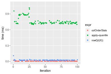
 Table: Benchmarking of colOrderStats() and rowOrderStats() on integer+10x10 data (original and transposed). The top panel shows times in milliseconds and the bottom panel shows relative times.
| expr | min | lq | mean | median | uq | max | |
|---|---|---|---|---|---|---|---|
| 1 | colOrderStats | 1.932 | 3.171 | 4.90543 | 5.677 | 6.0760 | 18.188 |
| 2 | rowOrderStats | 2.043 | 3.086 | 4.82545 | 5.679 | 6.0765 | 17.788 |
| expr | min | lq | mean | median | uq | max | |
|---|---|---|---|---|---|---|---|
| 1 | colOrderStats | 1.000000 | 1.0000000 | 1.0000000 | 1.000000 | 1.000000 | 1.0000000 |
| 2 | rowOrderStats | 1.057453 | 0.9731946 | 0.9836956 | 1.000352 | 1.000082 | 0.9780075 |
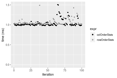
Figure: Benchmarking of colOrderStats() and rowOrderStats() on integer+10x10 data (original and transposed). Outliers are displayed as crosses. Times are in milliseconds.

> X <- data[["100x100"]]
> gc()
          used  (Mb) gc trigger  (Mb) max used  (Mb)
Ncells 3161481 168.9    5709258 305.0  5709258 305.0
Vcells 5858388  44.7   22267496 169.9 56666022 432.4
> probs <- 0.3
> which <- round(probs * nrow(X))
> colStats <- microbenchmark(colOrderStats = colOrderStats(X, which = which, na.rm = FALSE), `apply+quantile` = apply(X,
+     MARGIN = 2L, FUN = quantile, probs = probs, na.rm = FALSE, type = 3L), `rowQ(t(X))` = rowQ(t(X),
+     which = which), unit = "ms")
> X <- t(X)
> gc()
          used  (Mb) gc trigger  (Mb) max used  (Mb)
Ncells 3161471 168.9    5709258 305.0  5709258 305.0
Vcells 5863489  44.8   22267496 169.9 56666022 432.4
> rowStats <- microbenchmark(rowOrderStats = rowOrderStats(X, which = which, na.rm = FALSE), `apply+quantile` = apply(X,
+     MARGIN = 1L, FUN = quantile, probs = probs, na.rm = FALSE, type = 3L), rowQ = rowQ(X, which = which),
+     unit = "ms")
Table: Benchmarking of colOrderStats(), apply+quantile() and rowQ(t(X))() on integer+100x100 data. The top panel shows times in milliseconds and the bottom panel shows relative times.
| expr | min | lq | mean | median | uq | max | |
|---|---|---|---|---|---|---|---|
| 1 | colOrderStats | 0.100325 | 0.105361 | 0.1146209 | 0.1111180 | 0.116927 | 0.261677 |
| 3 | rowQ(t(X)) | 0.257913 | 0.265549 | 0.2889740 | 0.2801135 | 0.298563 | 0.722735 |
| 2 | apply+quantile | 7.159544 | 7.281613 | 7.9360339 | 7.4042465 | 7.797231 | 24.140317 |
| expr | min | lq | mean | median | uq | max | |
|---|---|---|---|---|---|---|---|
| 1 | colOrderStats | 1.000000 | 1.000000 | 1.000000 | 1.000000 | 1.000000 | 1.000000 |
| 3 | rowQ(t(X)) | 2.570775 | 2.520373 | 2.521128 | 2.520865 | 2.553414 | 2.761935 |
| 2 | apply+quantile | 71.363509 | 69.111090 | 69.237208 | 66.634087 | 66.684602 | 92.252345 |
Table: Benchmarking of rowOrderStats(), apply+quantile() and rowQ() on integer+100x100 data (transposed). The top panel shows times in milliseconds and the bottom panel shows relative times.
| expr | min | lq | mean | median | uq | max | |
|---|---|---|---|---|---|---|---|
| 1 | rowOrderStats | 0.102724 | 0.1060750 | 0.1124859 | 0.1105265 | 0.1167675 | 0.143676 |
| 3 | rowQ | 0.241839 | 0.2493755 | 0.2636848 | 0.2596140 | 0.2692875 | 0.325968 |
| 2 | apply+quantile | 7.175032 | 7.3049795 | 7.8897440 | 7.4196035 | 7.8356985 | 15.390523 |
| expr | min | lq | mean | median | uq | max | |
|---|---|---|---|---|---|---|---|
| 1 | rowOrderStats | 1.00000 | 1.000000 | 1.000000 | 1.000000 | 1.000000 | 1.000000 |
| 3 | rowQ | 2.35426 | 2.350936 | 2.344158 | 2.348885 | 2.306185 | 2.268771 |
| 2 | apply+quantile | 69.84767 | 68.866175 | 70.139824 | 67.129634 | 67.105132 | 107.119651 |
Figure: Benchmarking of colOrderStats(), apply+quantile() and rowQ(t(X))() on integer+100x100 data as well as rowOrderStats(), apply+quantile() and rowQ() on the same data transposed. Outliers are displayed as crosses. Times are in milliseconds.
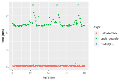
 Table: Benchmarking of colOrderStats() and rowOrderStats() on integer+100x100 data (original and transposed). The top panel shows times in milliseconds and the bottom panel shows relative times.
| expr | min | lq | mean | median | uq | max | |
|---|---|---|---|---|---|---|---|
| 2 | rowOrderStats | 102.724 | 106.075 | 112.4859 | 110.5265 | 116.7675 | 143.676 |
| 1 | colOrderStats | 100.325 | 105.361 | 114.6209 | 111.1180 | 116.9270 | 261.677 |
| expr | min | lq | mean | median | uq | max | |
|---|---|---|---|---|---|---|---|
| 2 | rowOrderStats | 1.0000000 | 1.0000000 | 1.00000 | 1.000000 | 1.000000 | 1.000000 |
| 1 | colOrderStats | 0.9766462 | 0.9932689 | 1.01898 | 1.005352 | 1.001366 | 1.821299 |
Figure: Benchmarking of colOrderStats() and rowOrderStats() on integer+100x100 data (original and transposed). Outliers are displayed as crosses. Times are in milliseconds.

> X <- data[["1000x10"]]
> gc()
          used  (Mb) gc trigger  (Mb) max used  (Mb)
Ncells 3162237 168.9    5709258 305.0  5709258 305.0
Vcells 5862171  44.8   22267496 169.9 56666022 432.4
> probs <- 0.3
> which <- round(probs * nrow(X))
> colStats <- microbenchmark(colOrderStats = colOrderStats(X, which = which, na.rm = FALSE), `apply+quantile` = apply(X,
+     MARGIN = 2L, FUN = quantile, probs = probs, na.rm = FALSE, type = 3L), `rowQ(t(X))` = rowQ(t(X),
+     which = which), unit = "ms")
> X <- t(X)
> gc()
          used  (Mb) gc trigger  (Mb) max used  (Mb)
Ncells 3162227 168.9    5709258 305.0  5709258 305.0
Vcells 5867272  44.8   22267496 169.9 56666022 432.4
> rowStats <- microbenchmark(rowOrderStats = rowOrderStats(X, which = which, na.rm = FALSE), `apply+quantile` = apply(X,
+     MARGIN = 1L, FUN = quantile, probs = probs, na.rm = FALSE, type = 3L), rowQ = rowQ(X, which = which),
+     unit = "ms")
Table: Benchmarking of colOrderStats(), apply+quantile() and rowQ(t(X))() on integer+1000x10 data. The top panel shows times in milliseconds and the bottom panel shows relative times.
| expr | min | lq | mean | median | uq | max | |
|---|---|---|---|---|---|---|---|
| 1 | colOrderStats | 0.088044 | 0.0918545 | 0.0941119 | 0.0944045 | 0.0953010 | 0.126456 |
| 3 | rowQ(t(X)) | 0.242794 | 0.2527940 | 0.2567904 | 0.2566280 | 0.2595115 | 0.291105 |
| 2 | apply+quantile | 1.002920 | 1.0377160 | 1.0578490 | 1.0530305 | 1.0669350 | 1.365025 |
| expr | min | lq | mean | median | uq | max | |
|---|---|---|---|---|---|---|---|
| 1 | colOrderStats | 1.000000 | 1.000000 | 1.000000 | 1.000000 | 1.000000 | 1.000000 |
| 3 | rowQ(t(X)) | 2.757644 | 2.752113 | 2.728564 | 2.718387 | 2.723072 | 2.302026 |
| 2 | apply+quantile | 11.391123 | 11.297389 | 11.240330 | 11.154452 | 11.195423 | 10.794466 |
Table: Benchmarking of rowOrderStats(), apply+quantile() and rowQ() on integer+1000x10 data (transposed). The top panel shows times in milliseconds and the bottom panel shows relative times.
| expr | min | lq | mean | median | uq | max | |
|---|---|---|---|---|---|---|---|
| 1 | rowOrderStats | 0.092744 | 0.0960315 | 0.0982252 | 0.0982475 | 0.0992300 | 0.137773 |
| 3 | rowQ | 0.228148 | 0.2358790 | 0.2401534 | 0.2402835 | 0.2433455 | 0.294290 |
| 2 | apply+quantile | 1.002051 | 1.0393100 | 1.0524716 | 1.0524280 | 1.0648230 | 1.234466 |
| expr | min | lq | mean | median | uq | max | |
|---|---|---|---|---|---|---|---|
| 1 | rowOrderStats | 1.000000 | 1.000000 | 1.000000 | 1.000000 | 1.000000 | 1.000000 |
| 3 | rowQ | 2.459976 | 2.456267 | 2.444928 | 2.445696 | 2.452338 | 2.136050 |
| 2 | apply+quantile | 10.804483 | 10.822595 | 10.714887 | 10.712008 | 10.730858 | 8.960145 |
Figure: Benchmarking of colOrderStats(), apply+quantile() and rowQ(t(X))() on integer+1000x10 data as well as rowOrderStats(), apply+quantile() and rowQ() on the same data transposed. Outliers are displayed as crosses. Times are in milliseconds.

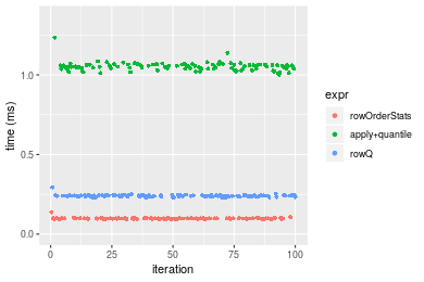 Table: Benchmarking of colOrderStats() and rowOrderStats() on integer+1000x10 data (original and transposed). The top panel shows times in milliseconds and the bottom panel shows relative times.
| expr | min | lq | mean | median | uq | max | |
|---|---|---|---|---|---|---|---|
| 1 | colOrderStats | 88.044 | 91.8545 | 94.11192 | 94.4045 | 95.301 | 126.456 |
| 2 | rowOrderStats | 92.744 | 96.0315 | 98.22517 | 98.2475 | 99.230 | 137.773 |
| expr | min | lq | mean | median | uq | max | |
|---|---|---|---|---|---|---|---|
| 1 | colOrderStats | 1.000000 | 1.000000 | 1.000000 | 1.000000 | 1.000000 | 1.000000 |
| 2 | rowOrderStats | 1.053382 | 1.045474 | 1.043706 | 1.040708 | 1.041227 | 1.089494 |
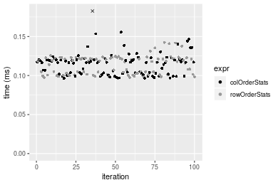
Figure: Benchmarking of colOrderStats() and rowOrderStats() on integer+1000x10 data (original and transposed). Outliers are displayed as crosses. Times are in milliseconds.

> X <- data[["10x1000"]]
> gc()
          used  (Mb) gc trigger  (Mb) max used  (Mb)
Ncells 3162442 168.9    5709258 305.0  5709258 305.0
Vcells 5862968  44.8   22267496 169.9 56666022 432.4
> probs <- 0.3
> which <- round(probs * nrow(X))
> colStats <- microbenchmark(colOrderStats = colOrderStats(X, which = which, na.rm = FALSE), `apply+quantile` = apply(X,
+     MARGIN = 2L, FUN = quantile, probs = probs, na.rm = FALSE, type = 3L), `rowQ(t(X))` = rowQ(t(X),
+     which = which), unit = "ms")
> X <- t(X)
> gc()
          used  (Mb) gc trigger  (Mb) max used  (Mb)
Ncells 3162432 168.9    5709258 305.0  5709258 305.0
Vcells 5868069  44.8   22267496 169.9 56666022 432.4
> rowStats <- microbenchmark(rowOrderStats = rowOrderStats(X, which = which, na.rm = FALSE), `apply+quantile` = apply(X,
+     MARGIN = 1L, FUN = quantile, probs = probs, na.rm = FALSE, type = 3L), rowQ = rowQ(X, which = which),
+     unit = "ms")
Table: Benchmarking of colOrderStats(), apply+quantile() and rowQ(t(X))() on integer+10x1000 data. The top panel shows times in milliseconds and the bottom panel shows relative times.
| expr | min | lq | mean | median | uq | max | |
|---|---|---|---|---|---|---|---|
| 1 | colOrderStats | 0.096422 | 0.102217 | 0.1151726 | 0.1168315 | 0.1203185 | 0.188983 |
| 3 | rowQ(t(X)) | 0.258851 | 0.269841 | 0.3028486 | 0.3116975 | 0.3231130 | 0.446715 |
| 2 | apply+quantile | 68.249799 | 69.420339 | 76.4880245 | 71.0519800 | 79.5367195 | 336.500526 |
| expr | min | lq | mean | median | uq | max | |
|---|---|---|---|---|---|---|---|
| 1 | colOrderStats | 1.000000 | 1.000000 | 1.00000 | 1.000000 | 1.000000 | 1.000000 |
| 3 | rowQ(t(X)) | 2.684564 | 2.639884 | 2.62952 | 2.667924 | 2.685481 | 2.363784 |
| 2 | apply+quantile | 707.823930 | 679.146708 | 664.11662 | 608.157731 | 661.051455 | 1780.586222 |
Table: Benchmarking of rowOrderStats(), apply+quantile() and rowQ() on integer+10x1000 data (transposed). The top panel shows times in milliseconds and the bottom panel shows relative times.
| expr | min | lq | mean | median | uq | max | |
|---|---|---|---|---|---|---|---|
| 1 | rowOrderStats | 0.097423 | 0.1014835 | 0.1138816 | 0.118211 | 0.122242 | 0.142445 |
| 3 | rowQ | 0.243022 | 0.2486300 | 0.2737372 | 0.276842 | 0.286358 | 0.602589 |
| 2 | apply+quantile | 68.140618 | 69.2765190 | 75.0524350 | 70.932610 | 81.330608 | 98.748079 |
| expr | min | lq | mean | median | uq | max | |
|---|---|---|---|---|---|---|---|
| 1 | rowOrderStats | 1.000000 | 1.000000 | 1.0000 | 1.000000 | 1.00000 | 1.000000 |
| 3 | rowQ | 2.494503 | 2.449955 | 2.4037 | 2.341931 | 2.34255 | 4.230327 |
| 2 | apply+quantile | 699.430504 | 682.638252 | 659.0389 | 600.050841 | 665.32459 | 693.236540 |
Figure: Benchmarking of colOrderStats(), apply+quantile() and rowQ(t(X))() on integer+10x1000 data as well as rowOrderStats(), apply+quantile() and rowQ() on the same data transposed. Outliers are displayed as crosses. Times are in milliseconds.

 Table: Benchmarking of colOrderStats() and rowOrderStats() on integer+10x1000 data (original and transposed). The top panel shows times in milliseconds and the bottom panel shows relative times.
| expr | min | lq | mean | median | uq | max | |
|---|---|---|---|---|---|---|---|
| 1 | colOrderStats | 96.422 | 102.2170 | 115.1726 | 116.8315 | 120.3185 | 188.983 |
| 2 | rowOrderStats | 97.423 | 101.4835 | 113.8816 | 118.2110 | 122.2420 | 142.445 |
| expr | min | lq | mean | median | uq | max | |
|---|---|---|---|---|---|---|---|
| 1 | colOrderStats | 1.000000 | 1.0000000 | 1.0000000 | 1.000000 | 1.000000 | 1.000000 |
| 2 | rowOrderStats | 1.010381 | 0.9928241 | 0.9887913 | 1.011808 | 1.015987 | 0.753745 |
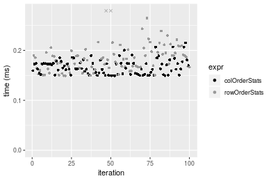
Figure: Benchmarking of colOrderStats() and rowOrderStats() on integer+10x1000 data (original and transposed). Outliers are displayed as crosses. Times are in milliseconds.
> X <- data[["100x1000"]]
> gc()
          used  (Mb) gc trigger  (Mb) max used  (Mb)
Ncells 3162655 169.0    5709258 305.0  5709258 305.0
Vcells 5863543  44.8   22267496 169.9 56666022 432.4
> probs <- 0.3
> which <- round(probs * nrow(X))
> colStats <- microbenchmark(colOrderStats = colOrderStats(X, which = which, na.rm = FALSE), `apply+quantile` = apply(X,
+     MARGIN = 2L, FUN = quantile, probs = probs, na.rm = FALSE, type = 3L), `rowQ(t(X))` = rowQ(t(X),
+     which = which), unit = "ms")
> X <- t(X)
> gc()
          used  (Mb) gc trigger  (Mb) max used  (Mb)
Ncells 3162645 169.0    5709258 305.0  5709258 305.0
Vcells 5913644  45.2   22267496 169.9 56666022 432.4
> rowStats <- microbenchmark(rowOrderStats = rowOrderStats(X, which = which, na.rm = FALSE), `apply+quantile` = apply(X,
+     MARGIN = 1L, FUN = quantile, probs = probs, na.rm = FALSE, type = 3L), rowQ = rowQ(X, which = which),
+     unit = "ms")
Table: Benchmarking of colOrderStats(), apply+quantile() and rowQ(t(X))() on integer+100x1000 data. The top panel shows times in milliseconds and the bottom panel shows relative times.
| expr | min | lq | mean | median | uq | max | |
|---|---|---|---|---|---|---|---|
| 1 | colOrderStats | 0.982719 | 0.992317 | 1.045162 | 1.006800 | 1.030469 | 1.506634 |
| 3 | rowQ(t(X)) | 2.397756 | 2.492323 | 2.623891 | 2.556417 | 2.612141 | 4.120215 |
| 2 | apply+quantile | 71.642484 | 73.291158 | 79.121191 | 74.524256 | 86.640305 | 105.794064 |
| expr | min | lq | mean | median | uq | max | |
|---|---|---|---|---|---|---|---|
| 1 | colOrderStats | 1.00000 | 1.00000 | 1.00000 | 1.000000 | 1.000000 | 1.000000 |
| 3 | rowQ(t(X)) | 2.43992 | 2.51162 | 2.51051 | 2.539151 | 2.534903 | 2.734715 |
| 2 | apply+quantile | 72.90231 | 73.85861 | 75.70230 | 74.020914 | 84.078476 | 70.218822 |
Table: Benchmarking of rowOrderStats(), apply+quantile() and rowQ() on integer+100x1000 data (transposed). The top panel shows times in milliseconds and the bottom panel shows relative times.
| expr | min | lq | mean | median | uq | max | |
|---|---|---|---|---|---|---|---|
| 1 | rowOrderStats | 1.011975 | 1.017653 | 1.064200 | 1.036333 | 1.059772 | 1.490149 |
| 3 | rowQ | 2.284843 | 2.362310 | 2.437772 | 2.405922 | 2.468891 | 2.934251 |
| 2 | apply+quantile | 70.957223 | 72.591067 | 78.896157 | 74.202615 | 86.877360 | 110.068004 |
| expr | min | lq | mean | median | uq | max | |
|---|---|---|---|---|---|---|---|
| 1 | rowOrderStats | 1.000000 | 1.000000 | 1.000000 | 1.000000 | 1.000000 | 1.000000 |
| 3 | rowQ | 2.257806 | 2.321332 | 2.290708 | 2.321572 | 2.329643 | 1.969099 |
| 2 | apply+quantile | 70.117565 | 71.331846 | 74.136581 | 71.601131 | 81.977407 | 73.863757 |
Figure: Benchmarking of colOrderStats(), apply+quantile() and rowQ(t(X))() on integer+100x1000 data as well as rowOrderStats(), apply+quantile() and rowQ() on the same data transposed. Outliers are displayed as crosses. Times are in milliseconds.

 Table: Benchmarking of colOrderStats() and rowOrderStats() on integer+100x1000 data (original and transposed). The top panel shows times in milliseconds and the bottom panel shows relative times.
| expr | min | lq | mean | median | uq | max | |
|---|---|---|---|---|---|---|---|
| 1 | colOrderStats | 982.719 | 992.317 | 1045.162 | 1006.800 | 1030.469 | 1506.634 |
| 2 | rowOrderStats | 1011.975 | 1017.653 | 1064.200 | 1036.333 | 1059.772 | 1490.149 |
| expr | min | lq | mean | median | uq | max | |
|---|---|---|---|---|---|---|---|
| 1 | colOrderStats | 1.00000 | 1.000000 | 1.000000 | 1.000000 | 1.000000 | 1.0000000 |
| 2 | rowOrderStats | 1.02977 | 1.025532 | 1.018215 | 1.029333 | 1.028436 | 0.9890584 |
Figure: Benchmarking of colOrderStats() and rowOrderStats() on integer+100x1000 data (original and transposed). Outliers are displayed as crosses. Times are in milliseconds.
> X <- data[["1000x100"]]
> gc()
          used  (Mb) gc trigger  (Mb) max used  (Mb)
Ncells 3162867 169.0    5709258 305.0  5709258 305.0
Vcells 5864231  44.8   22267496 169.9 56666022 432.4
> probs <- 0.3
> which <- round(probs * nrow(X))
> colStats <- microbenchmark(colOrderStats = colOrderStats(X, which = which, na.rm = FALSE), `apply+quantile` = apply(X,
+     MARGIN = 2L, FUN = quantile, probs = probs, na.rm = FALSE, type = 3L), `rowQ(t(X))` = rowQ(t(X),
+     which = which), unit = "ms")
> X <- t(X)
> gc()
          used  (Mb) gc trigger  (Mb) max used  (Mb)
Ncells 3162857 169.0    5709258 305.0  5709258 305.0
Vcells 5914332  45.2   22343563 170.5 56666022 432.4
> rowStats <- microbenchmark(rowOrderStats = rowOrderStats(X, which = which, na.rm = FALSE), `apply+quantile` = apply(X,
+     MARGIN = 1L, FUN = quantile, probs = probs, na.rm = FALSE, type = 3L), rowQ = rowQ(X, which = which),
+     unit = "ms")
Table: Benchmarking of colOrderStats(), apply+quantile() and rowQ(t(X))() on integer+1000x100 data. The top panel shows times in milliseconds and the bottom panel shows relative times.
| expr | min | lq | mean | median | uq | max | |
|---|---|---|---|---|---|---|---|
| 1 | colOrderStats | 0.908698 | 0.918584 | 0.9711281 | 0.9252755 | 0.940986 | 1.500015 |
| 3 | rowQ(t(X)) | 2.348175 | 2.451135 | 5.0738679 | 2.5224085 | 2.658630 | 246.989893 |
| 2 | apply+quantile | 9.547893 | 9.749097 | 10.3127077 | 9.8414515 | 10.013106 | 21.748900 |
| expr | min | lq | mean | median | uq | max | |
|---|---|---|---|---|---|---|---|
| 1 | colOrderStats | 1.000000 | 1.000000 | 1.000000 | 1.000000 | 1.000000 | 1.00000 |
| 3 | rowQ(t(X)) | 2.584109 | 2.668384 | 5.224715 | 2.726116 | 2.825366 | 164.65828 |
| 2 | apply+quantile | 10.507224 | 10.613179 | 10.619307 | 10.636239 | 10.641079 | 14.49912 |
Table: Benchmarking of rowOrderStats(), apply+quantile() and rowQ() on integer+1000x100 data (transposed). The top panel shows times in milliseconds and the bottom panel shows relative times.
| expr | min | lq | mean | median | uq | max | |
|---|---|---|---|---|---|---|---|
| 1 | rowOrderStats | 0.954094 | 0.9646065 | 1.019438 | 0.972211 | 0.992552 | 1.417984 |
| 3 | rowQ | 2.224715 | 2.3062425 | 2.513451 | 2.337960 | 2.369690 | 10.432955 |
| 2 | apply+quantile | 9.573497 | 9.7311070 | 10.058221 | 9.840734 | 9.990557 | 17.754467 |
| expr | min | lq | mean | median | uq | max | |
|---|---|---|---|---|---|---|---|
| 1 | rowOrderStats | 1.000000 | 1.000000 | 1.000000 | 1.000000 | 1.000000 | 1.000000 |
| 3 | rowQ | 2.331757 | 2.390864 | 2.465525 | 2.404787 | 2.387472 | 7.357597 |
| 2 | apply+quantile | 10.034123 | 10.088162 | 9.866433 | 10.122015 | 10.065525 | 12.520922 |
Figure: Benchmarking of colOrderStats(), apply+quantile() and rowQ(t(X))() on integer+1000x100 data as well as rowOrderStats(), apply+quantile() and rowQ() on the same data transposed. Outliers are displayed as crosses. Times are in milliseconds.
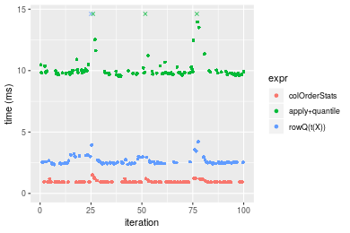
 Table: Benchmarking of colOrderStats() and rowOrderStats() on integer+1000x100 data (original and transposed). The top panel shows times in milliseconds and the bottom panel shows relative times.
| expr | min | lq | mean | median | uq | max | |
|---|---|---|---|---|---|---|---|
| 1 | colOrderStats | 908.698 | 918.5840 | 971.1281 | 925.2755 | 940.986 | 1500.015 |
| 2 | rowOrderStats | 954.094 | 964.6065 | 1019.4385 | 972.2110 | 992.552 | 1417.984 |
| expr | min | lq | mean | median | uq | max | |
|---|---|---|---|---|---|---|---|
| 1 | colOrderStats | 1.000000 | 1.000000 | 1.000000 | 1.000000 | 1.0000 | 1.0000000 |
| 2 | rowOrderStats | 1.049957 | 1.050102 | 1.049747 | 1.050726 | 1.0548 | 0.9453132 |
Figure: Benchmarking of colOrderStats() and rowOrderStats() on integer+1000x100 data (original and transposed). Outliers are displayed as crosses. Times are in milliseconds.

> rmatrix <- function(nrow, ncol, mode = c("logical", "double", "integer", "index"), range = c(-100,
+     +100), na_prob = 0) {
+     mode <- match.arg(mode)
+     n <- nrow * ncol
+     if (mode == "logical") {
+         x <- sample(c(FALSE, TRUE), size = n, replace = TRUE)
+     }     else if (mode == "index") {
+         x <- seq_len(n)
+         mode <- "integer"
+     }     else {
+         x <- runif(n, min = range[1], max = range[2])
+     }
+     storage.mode(x) <- mode
+     if (na_prob > 0)
+         x[sample(n, size = na_prob * n)] <- NA
+     dim(x) <- c(nrow, ncol)
+     x
+ }
> rmatrices <- function(scale = 10, seed = 1, ...) {
+     set.seed(seed)
+     data <- list()
+     data[[1]] <- rmatrix(nrow = scale * 1, ncol = scale * 1, ...)
+     data[[2]] <- rmatrix(nrow = scale * 10, ncol = scale * 10, ...)
+     data[[3]] <- rmatrix(nrow = scale * 100, ncol = scale * 1, ...)
+     data[[4]] <- t(data[[3]])
+     data[[5]] <- rmatrix(nrow = scale * 10, ncol = scale * 100, ...)
+     data[[6]] <- t(data[[5]])
+     names(data) <- sapply(data, FUN = function(x) paste(dim(x), collapse = "x"))
+     data
+ }
> data <- rmatrices(mode = mode)> X <- data[["10x10"]]
> gc()
used (Mb) gc trigger (Mb) max used (Mb)
Ncells 3163081 169.0 5709258 305.0 5709258 305.0
Vcells 5980119 45.7 22343563 170.5 56666022 432.4
> probs <- 0.3
> which <- round(probs * nrow(X))
> colStats <- microbenchmark(colOrderStats = colOrderStats(X, which = which, na.rm = FALSE), `apply+quantile` = apply(X,
+ MARGIN = 2L, FUN = quantile, probs = probs, na.rm = FALSE, type = 3L), `rowQ(t(X))` = rowQ(t(X),
+ which = which), unit = "ms")
> X <- t(X)
> gc()
used (Mb) gc trigger (Mb) max used (Mb)
Ncells 3163059 169.0 5709258 305.0 5709258 305.0
Vcells 5980300 45.7 22343563 170.5 56666022 432.4
> rowStats <- microbenchmark(rowOrderStats = rowOrderStats(X, which = which, na.rm = FALSE), `apply+quantile` = apply(X,
+ MARGIN = 1L, FUN = quantile, probs = probs, na.rm = FALSE, type = 3L), rowQ = rowQ(X, which = which),
+ unit = "ms")Table: Benchmarking of colOrderStats(), apply+quantile() and rowQ(t(X))() on double+10x10 data. The top panel shows times in milliseconds and the bottom panel shows relative times.
| expr | min | lq | mean | median | uq | max | |
|---|---|---|---|---|---|---|---|
| 1 | colOrderStats | 0.002342 | 0.0034530 | 0.0050972 | 0.0057735 | 0.0065100 | 0.017683 |
| 3 | rowQ(t(X)) | 0.007403 | 0.0093375 | 0.0130076 | 0.0112980 | 0.0155150 | 0.079125 |
| 2 | apply+quantile | 0.700793 | 0.7078400 | 0.7190105 | 0.7146930 | 0.7235135 | 0.981725 |
| expr | min | lq | mean | median | uq | max | |
|---|---|---|---|---|---|---|---|
| 1 | colOrderStats | 1.000000 | 1.00000 | 1.000000 | 1.000000 | 1.000000 | 1.000000 |
| 3 | rowQ(t(X)) | 3.160973 | 2.70417 | 2.551887 | 1.956872 | 2.383256 | 4.474637 |
| 2 | apply+quantile | 299.228437 | 204.99276 | 141.058783 | 123.788517 | 111.138786 | 55.518012 |
Table: Benchmarking of rowOrderStats(), apply+quantile() and rowQ() on double+10x10 data (transposed). The top panel shows times in milliseconds and the bottom panel shows relative times.
| expr | min | lq | mean | median | uq | max | |
|---|---|---|---|---|---|---|---|
| 3 | rowQ | 0.003801 | 0.0045715 | 0.0070744 | 0.0056585 | 0.0087095 | 0.054254 |
| 1 | rowOrderStats | 0.002495 | 0.0034090 | 0.0050627 | 0.0056910 | 0.0063535 | 0.019401 |
| 2 | apply+quantile | 0.698146 | 0.7050025 | 0.7144014 | 0.7106970 | 0.7175685 | 0.968225 |
| expr | min | lq | mean | median | uq | max | |
|---|---|---|---|---|---|---|---|
| 3 | rowQ | 1.0000000 | 1.0000000 | 1.0000000 | 1.000000 | 1.0000000 | 1.0000000 |
| 1 | rowOrderStats | 0.6564062 | 0.7457071 | 0.7156417 | 1.005744 | 0.7294908 | 0.3575958 |
| 2 | apply+quantile | 183.6742962 | 154.2168872 | 100.9847378 | 125.598127 | 82.3891727 | 17.8461496 |
Figure: Benchmarking of colOrderStats(), apply+quantile() and rowQ(t(X))() on double+10x10 data as well as rowOrderStats(), apply+quantile() and rowQ() on the same data transposed. Outliers are displayed as crosses. Times are in milliseconds.

 Table: Benchmarking of colOrderStats() and rowOrderStats() on double+10x10 data (original and transposed). The top panel shows times in milliseconds and the bottom panel shows relative times.
| expr | min | lq | mean | median | uq | max | |
|---|---|---|---|---|---|---|---|
| 2 | rowOrderStats | 2.495 | 3.409 | 5.06270 | 5.6910 | 6.3535 | 19.401 |
| 1 | colOrderStats | 2.342 | 3.453 | 5.09724 | 5.7735 | 6.5100 | 17.683 |
| expr | min | lq | mean | median | uq | max | |
|---|---|---|---|---|---|---|---|
| 2 | rowOrderStats | 1.0000000 | 1.000000 | 1.000000 | 1.000000 | 1.000000 | 1.0000000 |
| 1 | colOrderStats | 0.9386774 | 1.012907 | 1.006822 | 1.014497 | 1.024632 | 0.9114479 |
Figure: Benchmarking of colOrderStats() and rowOrderStats() on double+10x10 data (original and transposed). Outliers are displayed as crosses. Times are in milliseconds.

> X <- data[["100x100"]]
> gc()
          used  (Mb) gc trigger  (Mb) max used  (Mb)
Ncells 3163274 169.0    5709258 305.0  5709258 305.0
Vcells 5981105  45.7   22343563 170.5 56666022 432.4
> probs <- 0.3
> which <- round(probs * nrow(X))
> colStats <- microbenchmark(colOrderStats = colOrderStats(X, which = which, na.rm = FALSE), `apply+quantile` = apply(X,
+     MARGIN = 2L, FUN = quantile, probs = probs, na.rm = FALSE, type = 3L), `rowQ(t(X))` = rowQ(t(X),
+     which = which), unit = "ms")
> X <- t(X)
> gc()
          used  (Mb) gc trigger  (Mb) max used  (Mb)
Ncells 3163264 169.0    5709258 305.0  5709258 305.0
Vcells 5991206  45.8   22343563 170.5 56666022 432.4
> rowStats <- microbenchmark(rowOrderStats = rowOrderStats(X, which = which, na.rm = FALSE), `apply+quantile` = apply(X,
+     MARGIN = 1L, FUN = quantile, probs = probs, na.rm = FALSE, type = 3L), rowQ = rowQ(X, which = which),
+     unit = "ms")
Table: Benchmarking of colOrderStats(), apply+quantile() and rowQ(t(X))() on double+100x100 data. The top panel shows times in milliseconds and the bottom panel shows relative times.
| expr | min | lq | mean | median | uq | max | |
|---|---|---|---|---|---|---|---|
| 1 | colOrderStats | 0.151852 | 0.1541930 | 0.1640386 | 0.160511 | 0.1676685 | 0.211924 |
| 3 | rowQ(t(X)) | 0.233200 | 0.2365015 | 0.2516724 | 0.245102 | 0.2590480 | 0.339546 |
| 2 | apply+quantile | 7.209046 | 7.3151465 | 7.8090190 | 7.423569 | 7.6967770 | 16.133390 |
| expr | min | lq | mean | median | uq | max | |
|---|---|---|---|---|---|---|---|
| 1 | colOrderStats | 1.000000 | 1.000000 | 1.000000 | 1.000000 | 1.000000 | 1.000000 |
| 3 | rowQ(t(X)) | 1.535706 | 1.533802 | 1.534228 | 1.527011 | 1.545001 | 1.602207 |
| 2 | apply+quantile | 47.474159 | 47.441495 | 47.604780 | 46.249597 | 45.904729 | 76.128187 |
Table: Benchmarking of rowOrderStats(), apply+quantile() and rowQ() on double+100x100 data (transposed). The top panel shows times in milliseconds and the bottom panel shows relative times.
| expr | min | lq | mean | median | uq | max | |
|---|---|---|---|---|---|---|---|
| 1 | rowOrderStats | 0.153110 | 0.1548275 | 0.1636779 | 0.158818 | 0.1681450 | 0.211434 |
| 3 | rowQ | 0.177858 | 0.1796600 | 0.1923398 | 0.188050 | 0.1972395 | 0.270269 |
| 2 | apply+quantile | 7.216398 | 7.2831930 | 7.9174679 | 7.430089 | 7.8410540 | 16.829715 |
| expr | min | lq | mean | median | uq | max | |
|---|---|---|---|---|---|---|---|
| 1 | rowOrderStats | 1.000000 | 1.000000 | 1.000000 | 1.00000 | 1.000000 | 1.000000 |
| 3 | rowQ | 1.161635 | 1.160388 | 1.175112 | 1.18406 | 1.173032 | 1.278266 |
| 2 | apply+quantile | 47.132114 | 47.040694 | 48.372253 | 46.78367 | 46.632692 | 79.597960 |
Figure: Benchmarking of colOrderStats(), apply+quantile() and rowQ(t(X))() on double+100x100 data as well as rowOrderStats(), apply+quantile() and rowQ() on the same data transposed. Outliers are displayed as crosses. Times are in milliseconds.

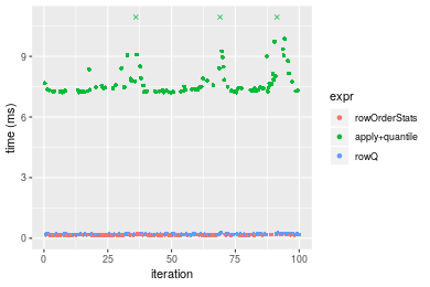 Table: Benchmarking of colOrderStats() and rowOrderStats() on double+100x100 data (original and transposed). The top panel shows times in milliseconds and the bottom panel shows relative times.
| expr | min | lq | mean | median | uq | max | |
|---|---|---|---|---|---|---|---|
| 2 | rowOrderStats | 153.110 | 154.8275 | 163.6779 | 158.818 | 168.1450 | 211.434 |
| 1 | colOrderStats | 151.852 | 154.1930 | 164.0385 | 160.511 | 167.6685 | 211.924 |
| expr | min | lq | mean | median | uq | max | |
|---|---|---|---|---|---|---|---|
| 2 | rowOrderStats | 1.0000000 | 1.0000000 | 1.000000 | 1.00000 | 1.0000000 | 1.000000 |
| 1 | colOrderStats | 0.9917837 | 0.9959019 | 1.002204 | 1.01066 | 0.9971661 | 1.002317 |
Figure: Benchmarking of colOrderStats() and rowOrderStats() on double+100x100 data (original and transposed). Outliers are displayed as crosses. Times are in milliseconds.

> X <- data[["1000x10"]]
> gc()
          used  (Mb) gc trigger  (Mb) max used  (Mb)
Ncells 3163487 169.0    5709258 305.0  5709258 305.0
Vcells 5982188  45.7   22343563 170.5 56666022 432.4
> probs <- 0.3
> which <- round(probs * nrow(X))
> colStats <- microbenchmark(colOrderStats = colOrderStats(X, which = which, na.rm = FALSE), `apply+quantile` = apply(X,
+     MARGIN = 2L, FUN = quantile, probs = probs, na.rm = FALSE, type = 3L), `rowQ(t(X))` = rowQ(t(X),
+     which = which), unit = "ms")
> X <- t(X)
> gc()
          used  (Mb) gc trigger  (Mb) max used  (Mb)
Ncells 3163477 169.0    5709258 305.0  5709258 305.0
Vcells 5992289  45.8   22343563 170.5 56666022 432.4
> rowStats <- microbenchmark(rowOrderStats = rowOrderStats(X, which = which, na.rm = FALSE), `apply+quantile` = apply(X,
+     MARGIN = 1L, FUN = quantile, probs = probs, na.rm = FALSE, type = 3L), rowQ = rowQ(X, which = which),
+     unit = "ms")
Table: Benchmarking of colOrderStats(), apply+quantile() and rowQ(t(X))() on double+1000x10 data. The top panel shows times in milliseconds and the bottom panel shows relative times.
| expr | min | lq | mean | median | uq | max | |
|---|---|---|---|---|---|---|---|
| 1 | colOrderStats | 0.137570 | 0.1398110 | 0.1443352 | 0.1422425 | 0.1461885 | 0.202188 |
| 3 | rowQ(t(X)) | 0.217051 | 0.2223905 | 0.2358092 | 0.2251030 | 0.2293180 | 0.517141 |
| 2 | apply+quantile | 1.112462 | 1.1351870 | 1.1728520 | 1.1503720 | 1.1706425 | 1.893386 |
| expr | min | lq | mean | median | uq | max | |
|---|---|---|---|---|---|---|---|
| 1 | colOrderStats | 1.000000 | 1.000000 | 1.000000 | 1.00000 | 1.000000 | 1.000000 |
| 3 | rowQ(t(X)) | 1.577749 | 1.590651 | 1.633761 | 1.58253 | 1.568646 | 2.557723 |
| 2 | apply+quantile | 8.086516 | 8.119440 | 8.125889 | 8.08740 | 8.007760 | 9.364483 |
Table: Benchmarking of rowOrderStats(), apply+quantile() and rowQ() on double+1000x10 data (transposed). The top panel shows times in milliseconds and the bottom panel shows relative times.
| expr | min | lq | mean | median | uq | max | |
|---|---|---|---|---|---|---|---|
| 1 | rowOrderStats | 0.142481 | 0.1474750 | 0.1708429 | 0.1713020 | 0.1895015 | 0.237021 |
| 3 | rowQ | 0.164252 | 0.1699545 | 0.1962792 | 0.1974145 | 0.2177905 | 0.278304 |
| 2 | apply+quantile | 1.079233 | 1.0967530 | 1.2899622 | 1.1835395 | 1.4491930 | 1.880415 |
| expr | min | lq | mean | median | uq | max | |
|---|---|---|---|---|---|---|---|
| 1 | rowOrderStats | 1.000000 | 1.000000 | 1.000000 | 1.000000 | 1.000000 | 1.000000 |
| 3 | rowQ | 1.152799 | 1.152429 | 1.148887 | 1.152435 | 1.149281 | 1.174174 |
| 2 | apply+quantile | 7.574575 | 7.436874 | 7.550574 | 6.909082 | 7.647396 | 7.933537 |
Figure: Benchmarking of colOrderStats(), apply+quantile() and rowQ(t(X))() on double+1000x10 data as well as rowOrderStats(), apply+quantile() and rowQ() on the same data transposed. Outliers are displayed as crosses. Times are in milliseconds.
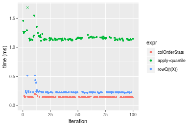
 Table: Benchmarking of colOrderStats() and rowOrderStats() on double+1000x10 data (original and transposed). The top panel shows times in milliseconds and the bottom panel shows relative times.
| expr | min | lq | mean | median | uq | max | |
|---|---|---|---|---|---|---|---|
| 1 | colOrderStats | 137.570 | 139.811 | 144.3352 | 142.2425 | 146.1885 | 202.188 |
| 2 | rowOrderStats | 142.481 | 147.475 | 170.8429 | 171.3020 | 189.5015 | 237.021 |
| expr | min | lq | mean | median | uq | max | |
|---|---|---|---|---|---|---|---|
| 1 | colOrderStats | 1.000000 | 1.000000 | 1.000000 | 1.000000 | 1.000000 | 1.00000 |
| 2 | rowOrderStats | 1.035698 | 1.054817 | 1.183654 | 1.204295 | 1.296282 | 1.17228 |
Figure: Benchmarking of colOrderStats() and rowOrderStats() on double+1000x10 data (original and transposed). Outliers are displayed as crosses. Times are in milliseconds.

> X <- data[["10x1000"]]
> gc()
          used  (Mb) gc trigger  (Mb) max used  (Mb)
Ncells 3163692 169.0    5709258 305.0  5709258 305.0
Vcells 5982324  45.7   22343563 170.5 56666022 432.4
> probs <- 0.3
> which <- round(probs * nrow(X))
> colStats <- microbenchmark(colOrderStats = colOrderStats(X, which = which, na.rm = FALSE), `apply+quantile` = apply(X,
+     MARGIN = 2L, FUN = quantile, probs = probs, na.rm = FALSE, type = 3L), `rowQ(t(X))` = rowQ(t(X),
+     which = which), unit = "ms")
> X <- t(X)
> gc()
          used  (Mb) gc trigger  (Mb) max used  (Mb)
Ncells 3163682 169.0    5709258 305.0  5709258 305.0
Vcells 5992425  45.8   22343563 170.5 56666022 432.4
> rowStats <- microbenchmark(rowOrderStats = rowOrderStats(X, which = which, na.rm = FALSE), `apply+quantile` = apply(X,
+     MARGIN = 1L, FUN = quantile, probs = probs, na.rm = FALSE, type = 3L), rowQ = rowQ(X, which = which),
+     unit = "ms")
Table: Benchmarking of colOrderStats(), apply+quantile() and rowQ(t(X))() on double+10x1000 data. The top panel shows times in milliseconds and the bottom panel shows relative times.
| expr | min | lq | mean | median | uq | max | |
|---|---|---|---|---|---|---|---|
| 1 | colOrderStats | 0.149321 | 0.1532270 | 0.1671298 | 0.163497 | 0.1740765 | 0.215217 |
| 3 | rowQ(t(X)) | 0.194589 | 0.1990095 | 0.2256560 | 0.231264 | 0.2459720 | 0.280529 |
| 2 | apply+quantile | 68.324530 | 69.5748805 | 75.6796908 | 70.979443 | 83.1125005 | 109.802889 |
| expr | min | lq | mean | median | uq | max | |
|---|---|---|---|---|---|---|---|
| 1 | colOrderStats | 1.000000 | 1.000000 | 1.000000 | 1.000000 | 1.000000 | 1.00000 |
| 3 | rowQ(t(X)) | 1.303159 | 1.298789 | 1.350184 | 1.414485 | 1.413011 | 1.30347 |
| 2 | apply+quantile | 457.568125 | 454.064104 | 452.819903 | 434.132999 | 477.448136 | 510.19617 |
Table: Benchmarking of rowOrderStats(), apply+quantile() and rowQ() on double+10x1000 data (transposed). The top panel shows times in milliseconds and the bottom panel shows relative times.
| expr | min | lq | mean | median | uq | max | |
|---|---|---|---|---|---|---|---|
| 1 | rowOrderStats | 0.149030 | 0.1664155 | 0.1850085 | 0.1819330 | 0.1961385 | 0.322571 |
| 3 | rowQ | 0.176522 | 0.1978705 | 0.2197706 | 0.2178195 | 0.2362470 | 0.319586 |
| 2 | apply+quantile | 68.027821 | 73.9741105 | 87.2590179 | 85.0304155 | 96.0258535 | 126.942856 |
| expr | min | lq | mean | median | uq | max | |
|---|---|---|---|---|---|---|---|
| 1 | rowOrderStats | 1.000000 | 1.000000 | 1.000000 | 1.000000 | 1.000000 | 1.0000000 |
| 3 | rowQ | 1.184473 | 1.189015 | 1.187895 | 1.197251 | 1.204491 | 0.9907462 |
| 2 | apply+quantile | 456.470650 | 444.514546 | 471.648646 | 467.372140 | 489.581869 | 393.5346203 |
Figure: Benchmarking of colOrderStats(), apply+quantile() and rowQ(t(X))() on double+10x1000 data as well as rowOrderStats(), apply+quantile() and rowQ() on the same data transposed. Outliers are displayed as crosses. Times are in milliseconds.

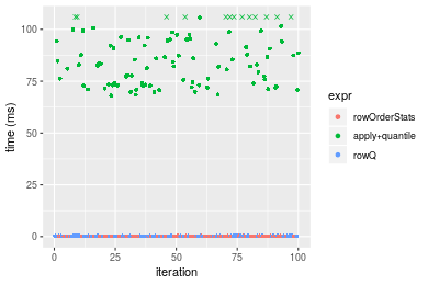 Table: Benchmarking of colOrderStats() and rowOrderStats() on double+10x1000 data (original and transposed). The top panel shows times in milliseconds and the bottom panel shows relative times.
| expr | min | lq | mean | median | uq | max | |
|---|---|---|---|---|---|---|---|
| 1 | colOrderStats | 149.321 | 153.2270 | 167.1298 | 163.497 | 174.0765 | 215.217 |
| 2 | rowOrderStats | 149.030 | 166.4155 | 185.0085 | 181.933 | 196.1385 | 322.571 |
| expr | min | lq | mean | median | uq | max | |
|---|---|---|---|---|---|---|---|
| 1 | colOrderStats | 1.0000000 | 1.000000 | 1.000000 | 1.000000 | 1.000000 | 1.000000 |
| 2 | rowOrderStats | 0.9980512 | 1.086072 | 1.106975 | 1.112761 | 1.126737 | 1.498817 |
Figure: Benchmarking of colOrderStats() and rowOrderStats() on double+10x1000 data (original and transposed). Outliers are displayed as crosses. Times are in milliseconds.
> X <- data[["100x1000"]]
> gc()
          used  (Mb) gc trigger  (Mb) max used  (Mb)
Ncells 3163905 169.0    5709258 305.0  5709258 305.0
Vcells 5983599  45.7   22343563 170.5 56666022 432.4
> probs <- 0.3
> which <- round(probs * nrow(X))
> colStats <- microbenchmark(colOrderStats = colOrderStats(X, which = which, na.rm = FALSE), `apply+quantile` = apply(X,
+     MARGIN = 2L, FUN = quantile, probs = probs, na.rm = FALSE, type = 3L), `rowQ(t(X))` = rowQ(t(X),
+     which = which), unit = "ms")
> X <- t(X)
> gc()
          used  (Mb) gc trigger  (Mb) max used  (Mb)
Ncells 3163895 169.0    5709258 305.0  5709258 305.0
Vcells 6083700  46.5   22343563 170.5 56666022 432.4
> rowStats <- microbenchmark(rowOrderStats = rowOrderStats(X, which = which, na.rm = FALSE), `apply+quantile` = apply(X,
+     MARGIN = 1L, FUN = quantile, probs = probs, na.rm = FALSE, type = 3L), rowQ = rowQ(X, which = which),
+     unit = "ms")
Table: Benchmarking of colOrderStats(), apply+quantile() and rowQ(t(X))() on double+100x1000 data. The top panel shows times in milliseconds and the bottom panel shows relative times.
| expr | min | lq | mean | median | uq | max | |
|---|---|---|---|---|---|---|---|
| 1 | colOrderStats | 1.493198 | 1.502794 | 1.575718 | 1.541372 | 1.606196 | 1.890651 |
| 3 | rowQ(t(X)) | 2.311336 | 2.393073 | 2.504513 | 2.453865 | 2.578567 | 3.096269 |
| 2 | apply+quantile | 72.706505 | 74.228516 | 83.233698 | 76.064604 | 87.782736 | 346.141771 |
| expr | min | lq | mean | median | uq | max | |
|---|---|---|---|---|---|---|---|
| 1 | colOrderStats | 1.00000 | 1.000000 | 1.000000 | 1.00000 | 1.000000 | 1.000000 |
| 3 | rowQ(t(X)) | 1.54791 | 1.592416 | 1.589442 | 1.59200 | 1.605387 | 1.637674 |
| 2 | apply+quantile | 48.69180 | 49.393673 | 52.822705 | 49.34863 | 54.652568 | 183.080733 |
Table: Benchmarking of rowOrderStats(), apply+quantile() and rowQ() on double+100x1000 data (transposed). The top panel shows times in milliseconds and the bottom panel shows relative times.
| expr | min | lq | mean | median | uq | max | |
|---|---|---|---|---|---|---|---|
| 1 | rowOrderStats | 1.513896 | 1.526642 | 1.615790 | 1.551529 | 1.640509 | 2.137383 |
| 3 | rowQ | 1.743967 | 1.751475 | 1.861983 | 1.797514 | 1.950642 | 2.402143 |
| 2 | apply+quantile | 71.923080 | 73.557554 | 81.185077 | 75.607957 | 87.977137 | 111.668584 |
| expr | min | lq | mean | median | uq | max | |
|---|---|---|---|---|---|---|---|
| 1 | rowOrderStats | 1.000000 | 1.000000 | 1.000000 | 1.000000 | 1.000000 | 1.000000 |
| 3 | rowQ | 1.151973 | 1.147273 | 1.152367 | 1.158544 | 1.189047 | 1.123871 |
| 2 | apply+quantile | 47.508600 | 48.182583 | 50.244826 | 48.731256 | 53.627951 | 52.245472 |
Figure: Benchmarking of colOrderStats(), apply+quantile() and rowQ(t(X))() on double+100x1000 data as well as rowOrderStats(), apply+quantile() and rowQ() on the same data transposed. Outliers are displayed as crosses. Times are in milliseconds.

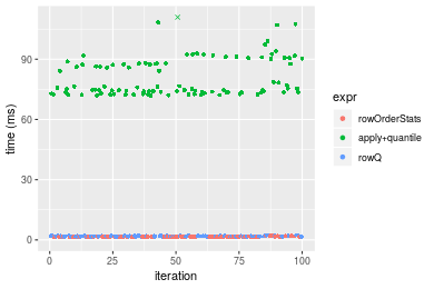 Table: Benchmarking of colOrderStats() and rowOrderStats() on double+100x1000 data (original and transposed). The top panel shows times in milliseconds and the bottom panel shows relative times.
| expr | min | lq | mean | median | uq | max | |
|---|---|---|---|---|---|---|---|
| 1 | colOrderStats | 1.493198 | 1.502794 | 1.575718 | 1.541372 | 1.606196 | 1.890651 |
| 2 | rowOrderStats | 1.513896 | 1.526642 | 1.615790 | 1.551529 | 1.640509 | 2.137383 |
| expr | min | lq | mean | median | uq | max | |
|---|---|---|---|---|---|---|---|
| 1 | colOrderStats | 1.000000 | 1.000000 | 1.000000 | 1.00000 | 1.000000 | 1.000000 |
| 2 | rowOrderStats | 1.013861 | 1.015869 | 1.025431 | 1.00659 | 1.021363 | 1.130501 |
Figure: Benchmarking of colOrderStats() and rowOrderStats() on double+100x1000 data (original and transposed). Outliers are displayed as crosses. Times are in milliseconds.

> X <- data[["1000x100"]]
> gc()
          used  (Mb) gc trigger  (Mb) max used  (Mb)
Ncells 3164117 169.0    5709258 305.0  5709258 305.0
Vcells 5983742  45.7   22343563 170.5 56666022 432.4
> probs <- 0.3
> which <- round(probs * nrow(X))
> colStats <- microbenchmark(colOrderStats = colOrderStats(X, which = which, na.rm = FALSE), `apply+quantile` = apply(X,
+     MARGIN = 2L, FUN = quantile, probs = probs, na.rm = FALSE, type = 3L), `rowQ(t(X))` = rowQ(t(X),
+     which = which), unit = "ms")
> X <- t(X)
> gc()
          used  (Mb) gc trigger  (Mb) max used  (Mb)
Ncells 3164107 169.0    5709258 305.0  5709258 305.0
Vcells 6083843  46.5   22343563 170.5 56666022 432.4
> rowStats <- microbenchmark(rowOrderStats = rowOrderStats(X, which = which, na.rm = FALSE), `apply+quantile` = apply(X,
+     MARGIN = 1L, FUN = quantile, probs = probs, na.rm = FALSE, type = 3L), rowQ = rowQ(X, which = which),
+     unit = "ms")
Table: Benchmarking of colOrderStats(), apply+quantile() and rowQ(t(X))() on double+1000x100 data. The top panel shows times in milliseconds and the bottom panel shows relative times.
| expr | min | lq | mean | median | uq | max | |
|---|---|---|---|---|---|---|---|
| 1 | colOrderStats | 1.493593 | 1.508093 | 1.619081 | 1.541671 | 1.624444 | 2.405428 |
| 3 | rowQ(t(X)) | 1.914679 | 1.997925 | 2.163334 | 2.077514 | 2.181479 | 3.283499 |
| 2 | apply+quantile | 10.443364 | 10.559361 | 11.512780 | 10.662634 | 11.467785 | 19.872912 |
| expr | min | lq | mean | median | uq | max | |
|---|---|---|---|---|---|---|---|
| 1 | colOrderStats | 1.000000 | 1.000000 | 1.000000 | 1.000000 | 1.000000 | 1.000000 |
| 3 | rowQ(t(X)) | 1.281928 | 1.324803 | 1.336149 | 1.347573 | 1.342908 | 1.365037 |
| 2 | apply+quantile | 6.992108 | 7.001799 | 7.110686 | 6.916284 | 7.059514 | 8.261695 |
Table: Benchmarking of rowOrderStats(), apply+quantile() and rowQ() on double+1000x100 data (transposed). The top panel shows times in milliseconds and the bottom panel shows relative times.
| expr | min | lq | mean | median | uq | max | |
|---|---|---|---|---|---|---|---|
| 1 | rowOrderStats | 1.548613 | 1.554814 | 1.612256 | 1.589789 | 1.624245 | 2.050989 |
| 3 | rowQ | 1.751948 | 1.762935 | 1.891934 | 1.787286 | 1.846548 | 9.923347 |
| 2 | apply+quantile | 10.460200 | 10.547797 | 10.970156 | 10.590273 | 10.709793 | 20.604903 |
| expr | min | lq | mean | median | uq | max | |
|---|---|---|---|---|---|---|---|
| 1 | rowOrderStats | 1.000000 | 1.000000 | 1.000000 | 1.000000 | 1.000000 | 1.000000 |
| 3 | rowQ | 1.131301 | 1.133856 | 1.173470 | 1.124229 | 1.136866 | 4.838323 |
| 2 | apply+quantile | 6.754560 | 6.783963 | 6.804227 | 6.661435 | 6.593708 | 10.046326 |
Figure: Benchmarking of colOrderStats(), apply+quantile() and rowQ(t(X))() on double+1000x100 data as well as rowOrderStats(), apply+quantile() and rowQ() on the same data transposed. Outliers are displayed as crosses. Times are in milliseconds.
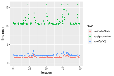
 Table: Benchmarking of colOrderStats() and rowOrderStats() on double+1000x100 data (original and transposed). The top panel shows times in milliseconds and the bottom panel shows relative times.
| expr | min | lq | mean | median | uq | max | |
|---|---|---|---|---|---|---|---|
| 1 | colOrderStats | 1.493593 | 1.508093 | 1.619081 | 1.541671 | 1.624444 | 2.405428 |
| 2 | rowOrderStats | 1.548613 | 1.554814 | 1.612256 | 1.589789 | 1.624245 | 2.050989 |
| expr | min | lq | mean | median | uq | max | |
|---|---|---|---|---|---|---|---|
| 1 | colOrderStats | 1.000000 | 1.00000 | 1.0000000 | 1.000000 | 1.0000000 | 1.0000000 |
| 2 | rowOrderStats | 1.036837 | 1.03098 | 0.9957845 | 1.031211 | 0.9998772 | 0.8526503 |
Figure: Benchmarking of colOrderStats() and rowOrderStats() on double+1000x100 data (original and transposed). Outliers are displayed as crosses. Times are in milliseconds.

R version 3.6.1 Patched (2019-08-27 r77078)
Platform: x86_64-pc-linux-gnu (64-bit)
Running under: Ubuntu 18.04.3 LTS

Matrix products: default
BLAS:   /home/hb/software/R-devel/R-3-6-branch/lib/R/lib/libRblas.so
LAPACK: /home/hb/software/R-devel/R-3-6-branch/lib/R/lib/libRlapack.so

locale:
 [1] LC_CTYPE=en_US.UTF-8       LC_NUMERIC=C
 [3] LC_TIME=en_US.UTF-8        LC_COLLATE=en_US.UTF-8
 [5] LC_MONETARY=en_US.UTF-8    LC_MESSAGES=en_US.UTF-8
 [7] LC_PAPER=en_US.UTF-8       LC_NAME=C
 [9] LC_ADDRESS=C               LC_TELEPHONE=C
[11] LC_MEASUREMENT=en_US.UTF-8 LC_IDENTIFICATION=C

attached base packages:
[1] stats     graphics  grDevices utils     datasets  methods   base

other attached packages:
[1] microbenchmark_1.4-6    matrixStats_0.55.0-9000 ggplot2_3.2.1
[4] knitr_1.24              R.devices_2.16.0        R.utils_2.9.0
[7] R.oo_1.22.0             R.methodsS3_1.7.1       history_0.0.0-9002

loaded via a namespace (and not attached):
 [1] Biobase_2.45.0       bit64_0.9-7          splines_3.6.1
 [4] network_1.15         assertthat_0.2.1     highr_0.8
 [7] stats4_3.6.1         blob_1.2.0           robustbase_0.93-5
[10] pillar_1.4.2         RSQLite_2.1.2        backports_1.1.4
[13] lattice_0.20-38      glue_1.3.1           digest_0.6.20
[16] colorspace_1.4-1     sandwich_2.5-1       Matrix_1.2-17
[19] XML_3.98-1.20        lpSolve_5.6.13.3     pkgconfig_2.0.2
[22] genefilter_1.66.0    purrr_0.3.2          ergm_3.10.4
[25] xtable_1.8-4         mvtnorm_1.0-11       scales_1.0.0
[28] tibble_2.1.3         annotate_1.62.0      IRanges_2.18.2
[31] TH.data_1.0-10       withr_2.1.2          BiocGenerics_0.30.0
[34] lazyeval_0.2.2       mime_0.7             survival_2.44-1.1
[37] magrittr_1.5         crayon_1.3.4         statnet.common_4.3.0
[40] memoise_1.1.0        laeken_0.5.0         R.cache_0.13.0
[43] MASS_7.3-51.4        R.rsp_0.43.1         tools_3.6.1
[46] multcomp_1.4-10      S4Vectors_0.22.1     trust_0.1-7
[49] munsell_0.5.0        AnnotationDbi_1.46.1 compiler_3.6.1
[52] rlang_0.4.0          grid_3.6.1           RCurl_1.95-4.12
[55] cwhmisc_6.6          rappdirs_0.3.1       labeling_0.3
[58] bitops_1.0-6         base64enc_0.1-3      boot_1.3-23
[61] gtable_0.3.0         codetools_0.2-16     DBI_1.0.0
[64] markdown_1.1         R6_2.4.0             zoo_1.8-6
[67] dplyr_0.8.3          bit_1.1-14           zeallot_0.1.0
[70] parallel_3.6.1       Rcpp_1.0.2           vctrs_0.2.0
[73] DEoptimR_1.0-8       tidyselect_0.2.5     xfun_0.9
[76] coda_0.19-3
Total processing time was 1.64 mins.
To reproduce this report, do:
html <- matrixStats:::benchmark('colOrderStats')Copyright Henrik Bengtsson. Last updated on 2019-09-10 20:48:22 (-0700 UTC). Powered by RSP.
<script> var link = document.createElement('link'); link.rel = 'icon'; link.href = "data:image/png;base64,iVBORw0KGgoAAAANSUhEUgAAACAAAAAgCAMAAABEpIrGAAAA21BMVEUAAAAAAP8AAP8AAP8AAP8AAP8AAP8AAP8AAP8AAP8AAP8AAP8AAP8AAP8AAP8AAP8AAP8AAP8AAP8AAP8AAP8AAP8AAP8AAP8AAP8AAP8AAP8AAP8AAP8AAP8AAP8AAP8AAP8AAP8AAP8AAP8AAP8AAP8AAP8AAP8AAP8AAP8BAf4CAv0DA/wdHeIeHuEfH+AgIN8hId4lJdomJtknJ9g+PsE/P8BAQL9yco10dIt1dYp3d4h4eIeVlWqWlmmXl2iYmGeZmWabm2Tn5xjo6Bfp6Rb39wj4+Af//wA2M9hbAAAASXRSTlMAAQIJCgsMJSYnKD4/QGRlZmhpamtsbautrrCxuru8y8zN5ebn6Pn6+///////////////////////////////////////////LsUNcQAAAS9JREFUOI29k21XgkAQhVcFytdSMqMETU26UVqGmpaiFbL//xc1cAhhwVNf6n5i5z67M2dmYOyfJZUqlVLhkKucG7cgmUZTybDz6g0iDeq51PUr37Ds2cy2/C9NeES5puDjxuUk1xnToZsg8pfA3avHQ3lLIi7iWRrkv/OYtkScxBIMgDee0ALoyxHQBJ68JLCjOtQIMIANF7QG9G9fNnHvisCHBVMKgSJgiz7nE+AoBKrAPA3MgepvgR9TSCasrCKH0eB1wBGBFdCO+nAGjMVGPcQb5bd6mQRegN6+1axOs9nGfYcCtfi4NQosdtH7dB+txFIpXQqN1p9B/asRHToyS0jRgpV7nk4nwcq1BJ+x3Gl/v7S9Wmpp/aGquum7w3ZDyrADFYrl8vHBH+ev9AUASW1dmU4h4wAAAABJRU5ErkJggg==" document.getElementsByTagName('head')[0].appendChild(link); </script>