Graphical model of SLAM

Based on two common used assumptions, namely the static world and the Markov assumption , the structure of SLAM problem can be described as a dynamic Bayesian network(DBN). Reference: Grisetti, Giorgio, et al. "A tutorial on graph-based SLAM." Intelligent Transportation Systems Magazine, IEEE 2.4 (2010): 31-43.

So the SLAM joint distribution of map and states is:

This representation is called the Rao-Blackwellization , which inspires us that the SLAM problem can be computed as two separate parts, constructing the map from known states and observations(map reconstruction) and find the most likely states given observations and control inputs(states alignment).

Map reconstruction

Data structure - grid map

We use grid maps to model the environment of our dataset. Grid maps discretize the environment into grid cells. Each cell stores the probability that this cell is occupied.

Algorithm

Reference:High resolution maps from wide angle sonar

Basic assumption:

1. Robot locations at each step is known;

2. Different cells are independent;

Probabilistic modeling

p(c) is the probability that the cell c is occupied by an obstacle. To generate the map, we need to calculate the probability of each cell based on background knowledge and . By Bayes' rule, we obtain

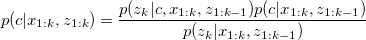
We assume that is independent from and and use Bayes' rule again, we obtain

Furthermore assume that does not carry any information about c if no observation , which leads to

Through some mathematical work, we finally obtain the iteration algorithm,

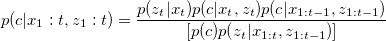
States alignment

Reference:Montemerlo, Michael, et al. "FastSLAM: A factored solution to the simultaneous localization and mapping problem." AAAI/IAAI. 2002.

Data structure

The basic idea of Rao-Blackwellized particle filter is to represent the joint distribution as a set of several particles. 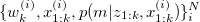Each particle represents an assumption for the robot path. The more the number of particles, the better the set can represent the distribution.

Algorithm

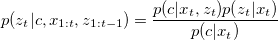
Assume we have N particles in total, at time k-1, the joint state is :

1. Draw a sample for new time step and add it to the particle history;

(1) Gaussian motion model ;

(2) Scan matching for the point cloud (ICP);

(3) Kalman filter or parameter-adaptive filter to correct the systematic error(left-directional bias here);

(4) Dynamic programming to find most possible pose - Viterbi algorithm;

(5) Dirichlet process or Gaussian mixture model(GMM) to estimate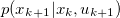

2. Renew sampled weight ;

3. Perform resampling;

4. For each particle, update the grid using the algorithm above.

Resampling

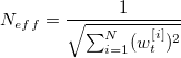
During resampling procedure, the particles with a low important weight are replaced by particles with a high weight. To do automatically resampling, we consider an efficient number of particles which was first introduced by Liu ("Metropolized independent sampling with comparisons to rejection sampling and importance sampling."):

Calculate the efficient number of particles, when it is smaller than , do stochastic universal resampling;

Scan matching

Iterative closest point(ICP)

http://www.princeton.edu/~hesun/icp_real.gif

https://youtu.be/_234wNp0ssU

Sum of gaussian optimization

Experiment

Here we set the proposal distribution as 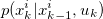, as FastSLAM 1.0 does in reference.

results before icp

result after icp

Problems without resampling:

As we only use current observation to do weight update, some bad particles can be over-qualified if they perform well in close states..