17 03 Decorrelating your data and dimension reduction - HannaAA17/Data-Scientist-With-Python-datacamp GitHub Wiki
Dimension reduction summarizes a dataset using its common occuring patterns. In this chapter, you'll learn about the most fundamental of dimension reduction techniques, "Principal Component Analysis" ("PCA"). PCA is often used before supervised learning to improve model performance and generalization. It can also be useful for unsupervised learning. For example, you'll employ a variant of PCA will allow you to cluster Wikipedia articles by their content!
01 Visualizing the PCA transformation
Principle Component Analysis
- Fundamental dimension reduction technique
- Step 1: decorrelation
- Step 2: reduce dimension
- PCA aligns data with axes
- Rotates data samples to be aligned with axes
- Shift data samples so that they have mean 0
- No information is lost
- PCA follows the fit/transform pattern
sklearncomponentfit()learns the transformation from given datatransform()applies the learned transformation to original/new data
Correlated data in nature
# Perform the necessary imports
import matplotlib.pyplot as plt
from scipy.stats import pearsonr

# Assign the 0th column of grains: width
width = grains[:,0]

# Assign the 1st column of grains: length
length = grains[:,1]

# Scatter plot width vs length
plt.scatter(width, length)
plt.axis('equal')
plt.show()

# Calculate the Pearson correlation
correlation, pvalue = pearsonr(width, length)

# Display the correlation
print(correlation)  # 0.8604149377143466
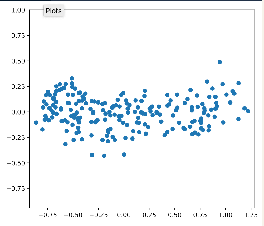
Decorrelating the grain measurements with PCA
# Import PCA
from sklearn.decomposition import PCA

# Create PCA instance: model
model = PCA()

# Apply the fit_transform method of model to grains: pca_features
pca_features = model.fit_transform(grains)

# Assign 0th column of pca_features: xs
xs = pca_features[:,0]

# Assign 1st column of pca_features: ys
ys = pca_features[:,1]

# Scatter plot xs vs ys
plt.scatter(xs, ys)
plt.axis('equal')
plt.show()

# Calculate the Pearson correlation of xs and ys
correlation, pvalue = pearsonr(xs, ys)

# Display the correlation
print(correlation) # around 0
PCA features are not correlated
Principal components
- "Principal components" = direction of variance
- PCA aligns principal components with the axes
- Available as
components_attribute of PCA object - Each row defines displacement from mean (vector)
02 Intrinsic dimension
- Number of features needed to approximate the data
- Essential idea behind dimension reduction
- What is the most compact representation of the samples?
- Can be detected with PCA
PCA identifies intrinsic dimension
- Intrinsic dimension = number of PCA features with significant variance
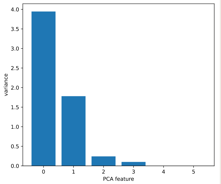
Plotting the variances of PCA features
- Intrinsic dimension can be ambiguous
# Perform the necessary imports
from sklearn.decomposition import PCA
from sklearn.preprocessing import StandardScaler
from sklearn.pipeline import make_pipeline
import matplotlib.pyplot as plt

# Create scaler: scaler
scaler = StandardScaler()

# Create a PCA instance: pca
pca = PCA()

# Create pipeline: pipeline
pipeline = make_pipeline(scaler, pca)

# Fit the pipeline to 'samples'
pipeline.fit(samples)

# Plot the explained variances
features = range(pca.n_components_)
plt.bar(features, pca.explained_variance_)
plt.xlabel('PCA feature')
plt.ylabel('variance')
plt.xticks(features)
plt.show()  # It looks like PCA features 0 and 1 have significant variance
03 Dimension reduction with PCA
Dimension reduction
- Represents same data using less feature
- Important part of machine-learning pipelines
- Can be performed using PCA
Dimension reduction with PCA
- Assumes the low variance features are "noise"
- TYPICALLY holds in practice
- And high variance features are informative
- Specify features to keep :
PCA(n_components=2)- Intrinsic dimension is a good choice
of the fish measurement
# Import PCA
from sklearn.decomposition import PCA

# Create a PCA model with 2 components: pca
pca = PCA(n_components = 2 )

# Fit the PCA instance to the scaled samples
pca.fit(scaled_samples)

# Transform the scaled samples: pca_features
pca_features = pca.transform(scaled_samples)

# Print the shape of pca_features
print(pca_features.shape)  # (85,2)
Word frequency arrays
- Rows represent documents, columns represent words
- Entries measure presence of each word in each documents
- Measure using "tf-idf"
- Sparse arrays and csr_matrix
- Sparse: most entries are zero
- Use
scipy.sparse.csr_matrixinstead of Numpy Array csr_matrixremembers only the non-zero entries (saves space!)
- TruncatedSVD and csr_matrix
PCAdoesn't supportcsr_matrix- Use
TruncatedSVDinstead
# Perform the necessary imports
from sklearn.decomposition import TruncatedSVD
from sklearn.cluster import KMeans
from sklearn.pipeline import make_pipeline
Import pandas as pd

# Create a TruncatedSVD instance: svd
svd = TruncatedSVD(n_components=50)

# Create a KMeans instance: kmeans
kmeans = KMeans(n_clusters=6)

# Create a pipeline: pipeline
pipeline = make_pipeline(svd, kmeans)

# Fit the pipeline to articles # type(articles): scipy.sparse.csr.csr_matrix
pipeline.fit(articles)

# Calculate the cluster labels: labels
labels = pipeline.predict(articles)

# Create a DataFrame aligning labels and titles: df
df = pd.DataFrame({'label': labels, 'article': titles})

# Display df sorted by cluster label
print(df.sort_values('label'))
      label                                        article
    59      0                                    Adam Levine
    57      0                          Red Hot Chili Peppers
    56      0                                       Skrillex
    55      0                                  Black Sabbath
    54      0                                 Arctic Monkeys
    53      0                                   Stevie Nicks
    52      0                                     The Wanted
    51      0                                     Nate Ruess
    50      0                                   Chad Kroeger
    58      0                                         Sepsis
    30      1                  France national football team
    31      1                              Cristiano Ronaldo
    32      1                                   Arsenal F.C.
    33      1                                 Radamel Falcao
    37      1                                       Football
    35      1                Colombia national football team
    36      1              2014 FIFA World Cup qualification
    38      1                                         Neymar
    39      1                                  Franck Ribéry
    34      1                             Zlatan Ibrahimović
    26      2                                     Mila Kunis
    28      2                                  Anne Hathaway
    27      2                                 Dakota Fanning
    25      2                                  Russell Crowe
    29      2                               Jennifer Aniston
    23      2                           Catherine Zeta-Jones
    22      2                              Denzel Washington
    21      2                             Michael Fassbender
    20      2                                 Angelina Jolie
    24      2                                   Jessica Biel
    10      3                                 Global warming
    11      3       Nationally Appropriate Mitigation Action
    13      3                               Connie Hedegaard
    14      3                                 Climate change
    12      3                                   Nigel Lawson
    16      3                                        350.org
    17      3  Greenhouse gas emissions by the United States
    18      3  2010 United Nations Climate Change Conference
    19      3  2007 United Nations Climate Change Conference
    15      3                                 Kyoto Protocol
...