16 03 Fine tuning your model - HannaAA17/Data-Scientist-With-Python-datacamp GitHub Wiki
01 Classification metrics
Accuracy
- Fraction of correctly classified samples
- vulnerable to class imbalance
Confusion matrix
| Predicted: Spam Email | Predicted: Real Email | |
|---|---|---|
| Actual: Spam | True Positive | False Negative |
| Actual: Real | False Positive | True Negative |
- Accuracy
(tp + tn) / (tp + tn + fp + fn)
- Precision
tp / (tp + fp )- High: not many real emails predicted as spam
- Recall
tp / (tp + fn)- High: predicted most spam emails correctly
- F1score
2 - (precision*recall) / (precision+recall)
Confusion matrix in scikit-learn
# necessary modules
from sklearn.metrics import classification_report
from sklearn.metrics import confusion_matrix
# Create training and test set
X_train, X_test, y_train, y_test = train_test_split(X, y, test_size=0.4, random_state = 42)

# Instantiate a k-NN classifier: knn
knn = KNeighborsClassifier(n_neighbors = 6)

# Fit the classifier to the training data
knn.fit(X_train, y_train)

# Predict the labels of the test data: y_pred
y_pred = knn.predict(X_test)

# Generate the confusion matrix and classification report
print(confusion_matrix(y_test, y_pred))
print(classification_report(y_test, y_pred))
[[176  30]
 [ 52  50]]
             precision    recall  f1-score   support

          0       0.77      0.85      0.81       206
          1       0.62      0.49      0.55       102

avg / total       0.72      0.73      0.72       308
02 Logistic Regression and the ROC curve
Logistic Regression for binary classification
- outputs probabilities
- If 'p' is greater than 0.5: The data is labeled '1, otherwise 0
- threshold here : 0.5
Logistic regression in scikit-learn
- module
from sklearn.linear_model import LogisticRegression
- fit, predict etc. just like other models
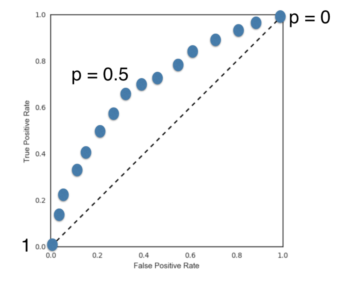
The ROC curve
- What happens if we vary the threshold?
- True Positive Rate = Recall
- False Positive Rate = FP / (FP + TN)
Say you have a binary classifier that in fact is just randomly making guesses. It would be correct approximately 50% of the time, and the resulting ROC curve would be a diagonal line in which the True Positive Rate and False Positive Rate are always equal.
Plot an ROC curve
# Import necessary modules
from sklearn.metrics import roc_curve

# Compute predicted probabilities: y_pred_prob
y_pred_prob = logreg.predict_proba(X_test)[:,1]

# Generate ROC curve values: fpr, tpr, thresholds
fpr, tpr, thresholds = roc_curve(y_test, y_pred_prob)

# Plot ROC curve
plt.plot([0, 1], [0, 1], 'k--')
plt.plot(fpr, tpr)
plt.xlabel('False Positive Rate')
plt.ylabel('True Positive Rate')
plt.title('ROC Curve')
plt.show()
03 Area under the ROC curve - AUC
- Larger area under the ROC curve.
from sklearn.metrics import roc_auc_score
# Import necessary modules
from sklearn.metrics import roc_auc_score
from sklearn.model_selection import cross_val_score

# Compute predicted probabilities: y_pred_prob
y_pred_prob = logreg.predict_proba(X_test)[:,1]

# Compute and print AUC score
print("AUC: {}".format(roc_auc_score(y_test, y_pred_prob)))

# Compute cross-validated AUC scores: cv_auc
cv_auc = cross_val_score(logreg, X, y, cv=5, scoring='roc_auc')

# Print list of AUC scores
print("AUC scores computed using 5-fold cross-validation: {}".format(cv_auc))
04 Hyperparameter tuning
- Parameters like alpha in Ridge/lasso regression and k in KNN
- These parameters need to be specified before fitting a model
- Try a bunch of different hyperparameter values and use cross-validation to choose the best performing one.
Grid search cross-validation
- Combination of all possible values - setup the hyperparameter grid: a dictionary of possible values - instantiate the GridSearchCV object with the classifier, param_grid and cv - fit the model
GridSearchCVinsklearn.model_selection-.best_params_&.best_score_
# Import necessary modules
from sklearn.linear_model import LogisticRegression
from sklearn.model_selection import GridSearchCV

# Setup the hyperparameter grid
c_space = np.logspace(-5, 8, 15)
param_grid = {'C': c_space}

# Instantiate a logistic regression classifier: logreg
logreg = LogisticRegression()

# Instantiate the GridSearchCV object: logreg_cv
logreg_cv = GridSearchCV(logreg, param_grid, cv=5)

# Fit it to the data
logreg_cv.fit(X, y)

# Print the tuned parameters and score
print("Tuned Logistic Regression Parameters: {}".format(logreg_cv.best_params_))
print("Best score is {}".format(logreg_cv.best_score_))
RandomizedSearchCV
GridSearchCV can be computationally expensive, especially if you are searching over a large hyperparameter space and dealing with multiple hyperparameters. A solution to this is to use RandomizedSearchCV, in which not all hyperparameter values are tried out. Instead, a fixed number of hyperparameter settings is sampled from specified probability distributions.
# Import necessary modules
from scipy.stats import randint
from sklearn.tree import DecisionTreeClassifier
from sklearn.model_selection import RandomizedSearchCV

# Setup the parameters and distributions to sample from: param_dist
param_dist = {"max_depth": [3, None],
              "max_features": randint(1, 9),
              "min_samples_leaf": randint(1, 9),
              "criterion": ["gini", "entropy"]}

# Instantiate a Decision Tree classifier: tree
tree = DecisionTreeClassifier()

# Instantiate the RandomizedSearchCV object: tree_cv
tree_cv = RandomizedSearchCV(tree, param_dist, cv=5)

# Fit it to the data
tree_cv.fit(X, y)

# Print the tuned parameters and score
print("Tuned Decision Tree Parameters: {}".format(tree_cv.best_params_))
print("Best score is {}".format(tree_cv.best_score_))
05 Hold-out set for final evaluation
- To see how well can the model perform on never before seen data
- Split data into training and hold-out set at the beginning
- Perform grid search cross-validation on training set
- Choose best hyperparameters and evaluate on hand-out set
Elastic net regularization is a combination of lasso(L1) and ridge(L2).
# Import necessary modules
from sklearn.linear_model import ElasticNet
from sklearn.metrics import mean_squared_error
from sklearn.model_selection import GridSearchCV, train_test_split


# Create train and test sets
X_train, X_test, y_train, y_test = train_test_split(X, y, test_size = 0.4, random_state = 42)

# Create the hyperparameter grid
l1_space = np.linspace(0, 1, 30)
param_grid = {'l1_ratio': l1_space}

# Instantiate the ElasticNet regressor: elastic_net
elastic_net = ElasticNet()

# Setup the GridSearchCV object: gm_cv
gm_cv = GridSearchCV(elastic_net, param_grid, cv=5)

# Fit it to the training data
gm_cv.fit(X_train, y_train)

# Predict on the test set and compute metrics
y_pred = gm_cv.predict(X_test)
r2 = gm_cv.score(X_test, y_test)
mse = mean_squared_error(y_test, y_pred)
print("Tuned ElasticNet l1 ratio: {}".format(gm_cv.best_params_))
print("Tuned ElasticNet R squared: {}".format(r2))
print("Tuned ElasticNet MSE: {}".format(mse))