16 02 Regression - HannaAA17/Data-Scientist-With-Python-datacamp GitHub Wiki
01 Intro to regression
Importing data for linear regression
Before that, however, you need to import the data and get it into the form needed by scikit-learn. This involves creating feature and target variable arrays. Furthermore, since you are going to use only one feature to begin with, you need to do some reshaping using NumPy's .reshape() method.
# Import numpy and pandas
import numpy as np
import pandas as pd

# Read the CSV file into a DataFrame: df
df = pd.read_csv('gapminder.csv')

# Create arrays for features and target variable
y = df['life'].values
X = df['fertility'].values

# Print the dimensions of X and y before reshaping
print("Dimensions of y before reshaping: {}".format(y.shape))  # (139, )
print("Dimensions of X before reshaping: {}".format(X.shape))

# Reshape X and y
y = y.reshape(-1, 1)
X = X.reshape(-1, 1)

# Print the dimensions of X and y after reshaping
print("Dimensions of y after reshaping: {}".format(y.shape)) # (139, 1)
print("Dimensions of X after reshaping: {}".format(X.shape))
02 The basics of linear regression
from sklearn.linear_model import LinearRegression
# Import necessary modules
from sklearn.linear_model import LinearRegression
from sklearn.metrics import mean_squared_error
from sklearn.model_selection import train_test_split

# Create training and test sets
X_train, X_test, y_train, y_test = train_test_split(X, y, test_size = 0.3, random_state=42)

# Create the regressor: reg_all
reg_all = LinearRegression()

# Fit the regressor to the training data
reg_all.fit(X_train, y_train)

# Predict on the test data: y_pred
y_pred = reg_all.predict(X_test)

# Compute and print R^2 and RMSE
print("R^2: {}".format(reg_all.score(X_test, y_test)))
rmse = np.sqrt(mean_squared_error(y_test, y_pred))
print("Root Mean Squared Error: {}".format(rmse))
03 Cross-validation motivation
- Model performance is dependent on way the data is split
- Not representative of the model's ability to generalize
- k-fold CV
- more folds = more computationally expensive
from sklearn.model_selection import cross_val_scorecv_results = cross_val_score(reg, X, y, cv=5)
# Import the necessary modules
from sklearn.linear_model import LinearRegression
from sklearn.model_selection import cross_val_score

# Create a linear regression object: reg
reg = LinearRegression()

# Compute 5-fold cross-validation scores: cv_scores
cv_scores = cross_val_score(reg, X, y , cv=5)

# Print the 5-fold cross-validation scores
print(cv_scores)

print("Average 5-Fold CV Score: {}".format(np.mean(cv_scores)))
04 Regularized regression
Why
- Linear regression minimizes a loss function
- It chooses a coefficient for each feature
- Large coefficient can lead to overfitting
- Penalizing large coefficients: Regularization
Ridge regression
Loss function = OLS loss function + Alpha * sum(ai^2))- Alpha: Parameter we need to choose
- 0: get back OLS, can lead to overfitting
- Very high alpha: can lead to underfitting
from sklearn,linear_model import Ridgeridge = Ridge(alpha=0.1, normalize = True)
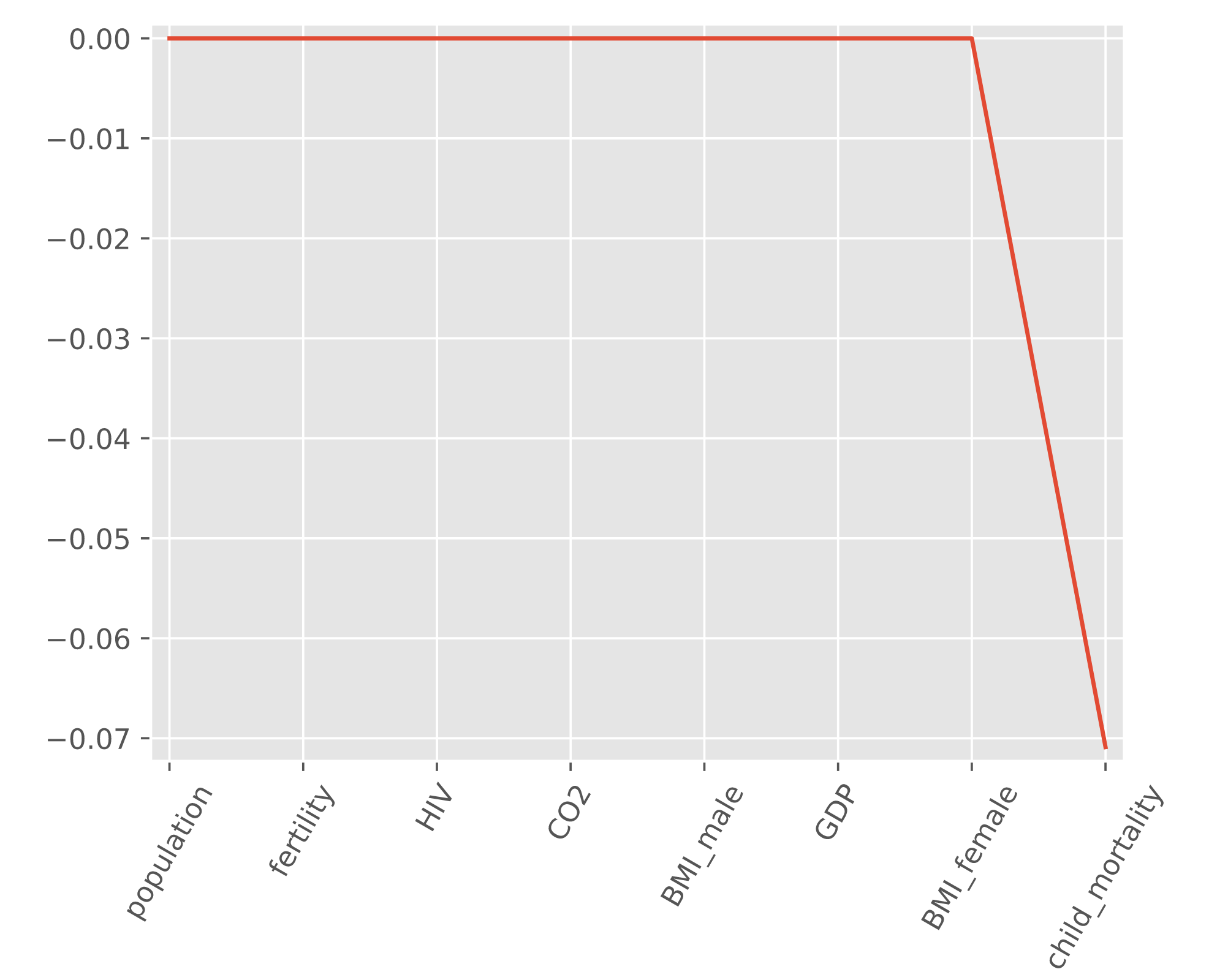
Lasso regression
Loss function = OLS loss function + Alpha * sum(abs(ai)))- Useful for selecting important features of a dataset - Shrinks the coefs of less important features to 0
from sklearn,linear_model import Lassolasso = Lasso(alpha=0.1, normalize = True)
- Lasso is great for feature selection, but when building regression models, Ridge regression should be your first choice.
# Import Lasso
from sklearn.linear_model import Lasso

# Instantiate a lasso regressor: lasso
lasso = Lasso(alpha=0.4 , normalize=True)

# Fit the regressor to the data
lasso.fit(X,y)

# Compute and print the coefficients
lasso_coef = lasso.coef_
print(lasso_coef)

# Plot the coefficients
plt.plot(range(len(df_columns)), lasso_coef)
plt.xticks(range(len(df_columns)), df_columns.values, rotation=60)
plt.margins(0.02)
plt.show()