15 02 Statistical Thinking in Python (Part 2) - HannaAA17/Data-Scientist-With-Python-datacamp GitHub Wiki
01 Parameter estimation by optimization
Optimal parameters
- Parameter values that bring the model in closest agreement with the data.
- Overlay the theoretical CDF with the ECDF from the data.
- This helps you to verify that the Exponential distribution describes the observed data.
- Packages to do statistical inference
- scipy.stats
- statsmodels
- hacker stats with numpy
Linear regression by least squares
- The process of finding the parameters for which the sum of the squares of the residuals is minimal.
np.polyfit(x, y ,1)slope, intercept = np.polyfit(x, y, 1)
# Plot the illiteracy rate versus fertility
_ = plt.plot(illiteracy, fertility, marker='.', linestyle='none')
plt.margins(0.02)
_ = plt.xlabel('percent illiterate')
_ = plt.ylabel('fertility')

# Perform a linear regression using np.polyfit(): a, b
a, b = np.polyfit(illiteracy, fertility, 1)

# Print the results to the screen
print('slope =', a, 'children per woman / percent illiterate')
print('intercept =', b, 'children per woman')

# Make theoretical line to plot
x = np.array([0,100])
y = a * x + b

# Add regression line to your plot
_ = plt.plot(x, y)

# Draw the plot
plt.show()
The importance of EDA: Anscombe's quartet
02 Bootstrap confidence intervals
Generating bootstrap replicates
- Bootstrapping: The use of resampled data to perform statistical inference.
- Bootstrap sample: A resampled array of the data.
- Sampling with replacement.
- Bootstrap replicates: A statistic computed from a resampled array (e.g. mean)
- Resampling engine:
np.random.choicenp.random.choice([1,2,3,4,5], size=5)- e.g:
array([5, 3, 5, 5, 2])
Bootstrap confidence interval
In fact, it can be shown theoretically that under not-too-restrictive conditions, the value of the mean will always be Normally distributed. (This does not hold in general, just for the mean and a few other statistics.)
- Step 1: Generate (many) bootstrap replicates
def draw_bs_reps(data, func, size=1):
    """Draw bootstrap replicates."""

    # Initialize array of replicates: bs_replicates
    bs_replicates = np.empty(size)

    # Generate replicates
    for i in range(size):
        bs_sample = np.random.choice(data, len(data))
        bs_replicates[i] = func(bs_sample)

    return bs_replicates
- Step 2: Plot a histogram of bootstrap replicates
- Step 3: Confidence interval
np.percentile(bs_replicates, [2.5, 97.5])
Pairs bootstrap
Non parametric inference
- Make no assumptions about the model or probability distribution underlying the data Pairs bootstrap for linear regression
- Resample data in pairs
- Compute slope and intercept from resampled data
- Each slope and intercept is a bootstrap replicate
- Compute confidence intervals from percentiles
A function to do pair bootstrap
def draw_bs_pairs_linreg(x, y, size=1):
    """Perform pairs bootstrap for linear regression."""

    # Set up array of indices to sample from: inds
    inds = np.arange(0,len(x))

    # Initialize replicates: bs_slope_reps, bs_intercept_reps
    bs_slope_reps = np.empty(size)
    bs_intercept_reps = np.empty(size)

    # Generate replicates
    for i in range(size):
        bs_inds = np.random.choice(inds, size=len(inds))
        bs_x, bs_y = x[bs_inds], y[bs_inds]
        bs_slope_reps[i], bs_intercept_reps[i] = np.polyfit(bs_x, bs_y, 1)

    return bs_slope_reps, bs_intercept_reps
03 Introduction to hypothesis testing
Formulating and simulating a hypothesis
Hypothesis testing
- Assessment of how reasonable the observed data are assuming a hypothesis is true.
Null hypothesis
- Another name for the hypothesis you are testing.
Permutation
- Random reordering of entries in an array.
- Permutation sampling is a great way to simulate the hypothesis that two variables have identical probability distributions.
- A function to generate a permutation sample from two data sets.
def permutation_sample(data1, data2):
    """Generate a permutation sample from two data sets."""

    # Concatenate the data sets: data
    data = np.concatenate((data1, data2))

    # Permute the concatenated array: permuted_data
    permuted_data = np.random.permutation(data)

    # Split the permuted array into two: perm_sample_1, perm_sample_2
    perm_sample_1 = permuted_data[:len(data1)]
    perm_sample_2 = permuted_data[len(data1):]

    return perm_sample_1, perm_sample_2
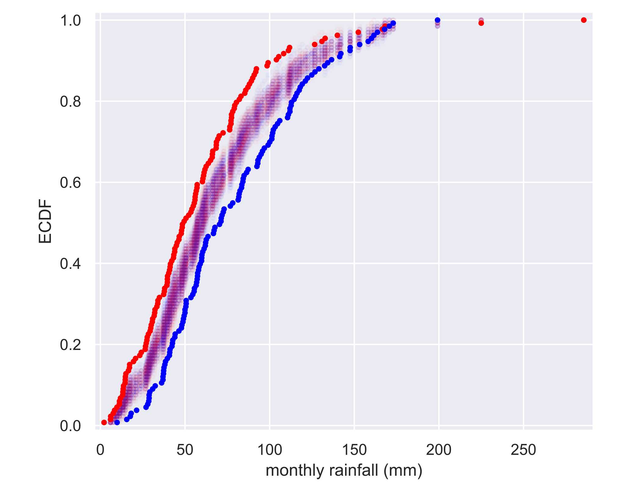
visualizing permutation sampling
for _ in range(50):
    # Generate permutation samples
    perm_sample_1, perm_sample_2 = permutation_sample(rain_june, rain_november)


    # Compute ECDFs
    x_1, y_1 = ecdf(perm_sample_1)
    x_2, y_2 = ecdf(perm_sample_2)

    # Plot ECDFs of permutation sample
    _ = plt.plot(x_1, y_1, marker='.', linestyle='none',
                 color='red', alpha=0.02)
    _ = plt.plot(x_2, y_2, marker='.', linestyle='none',
                 color='blue', alpha=0.02)

# Create and plot ECDFs from original data
x_1, y_1 = ecdf(rain_june)
x_2, y_2 = ecdf(rain_november)
_ = plt.plot(x_1, y_1, marker='.', linestyle='none', color='red')
_ = plt.plot(x_2, y_2, marker='.', linestyle='none', color='blue')

# Label axes, set margin, and show plot
plt.margins(0.02)
_ = plt.xlabel('monthly rainfall (mm)')
_ = plt.ylabel('ECDF')
plt.show()
Apparently, not the same distribution
Test statistics and p-values
Test statistic
- A single number that can be computed from observed data and from data you simulate under the null hypothesis.
- It serves as a basis of comparison between the two.
p-value
- The probability of obtaining a value of your test statistic that is at least as extreme as what was observed, under the assumption that the null hypothesis is true.
- NOT the probability that the null hypothesis is true.
Statistical significance
- Determined by the smallness of a p-value.
statistical significance vs. practical significance
- Remember: statistical significance (that is, low p-values) and practical significance, whether or not the difference of the data from the null hypothesis matters for practical considerations, are two different things.
Generate permutation replicates
def draw_perm_reps(data_1, data_2, func, size=1):
    """Generate multiple permutation replicates."""

    # Initialize array of replicates: perm_replicates
    perm_replicates = np.empty(size)

    for i in range(size):
        # Generate permutation sample
        perm_sample_1, perm_sample_2 = permutation_sample(data_1, data_2)

        # Compute the test statistic
        perm_replicates[i] = func(perm_sample_1, perm_sample_2)

    return perm_replicates
Bootstrap hypothesis tests
Pipeline for hypothesis testing
- Clearly state the null hypothesis
- Define test statistic
- Generate many sets of simulated data assuming the null hypothesis is true
- Compute the test statistic for each simulated data set
- The p-value
One sample test
- Compare one set of data to a single number
- The mean of dataset A is equal to number B.
To set up the bootstrap hypothesis test, you will take the mean as our test statistic. Remember, your goal is to calculate the probability of getting a mean impact force less than or equal to what was observed for Frog B if the hypothesis that the true mean of Frog B's impact forces is equal to that of Frog C is true. You first translate all of the data of Frog B such that the mean is 0.55 N. This involves adding the mean force of Frog C and subtracting the mean force of Frog B from each measurement of Frog B. This leaves other properties of Frog B's distribution, such as the variance, unchanged.
# Make an array of translated impact forces: translated_force_b
translated_force_b = force_b - force_b.mean() + 0.55

# Take bootstrap replicates of Frog B's translated impact forces: bs_replicates
bs_replicates = draw_bs_reps(translated_force_b, np.mean , 10000)

# Compute fraction of replicates that are less than the observed Frog B force: p
p = np.sum(bs_replicates <= np.mean(force_b)) / 10000

# Print the p-value
print('p = ', p)  #p =  0.0046
The low p-value suggests that the null hypothesis that Frog B and Frog C have the same mean impact force is false.
Two sample test
- Compare two sets of data
- The mean of dataset A = The mean of dataset B (but not exactly the same distribution)
04 Hypothesis test examples
A/B testing
- Used by organizations to see if a strategy change gives a better result.
- Null hypothesis: the test statistic is impervious to the change.
Test of correlation
- Posit null hypothesis: the two variables are completely uncorrelated
- Simulate data assuming null hypothesis is true
- Use Pearson correlation as test statistic
- Compute p-value
To do so, permute the illiteracy values but leave the fertility values fixed. This simulates the hypothesis that they are totally independent of each other. For each permutation, compute the Pearson correlation coefficient and assess how many of your permutation replicates have a Pearson correlation coefficient greater than the observed one.
# Compute observed correlation: r_obs
r_obs = pearson_r(illiteracy, fertility)

# Initialize permutation replicates: perm_replicates
perm_replicates = np.empty(10000)

# Draw replicates
for i in range(10000):
    # Permute illiteracy measurments: illiteracy_permuted
    illiteracy_permuted = np.random.permutation(illiteracy)

    # Compute Pearson correlation
    perm_replicates[i] = pearson_r(illiteracy_permuted, fertility)

# Compute p-value: p
p = np.sum(perm_replicates >= r_obs)/len(perm_replicates)
print('p-val =', p)