The full Kraus-Turner slab mixed layer model (KTA) carries the mixed layer thickness as a full prognostic variable. Since the mixed layer base (MLB) does not coincide with a model interface as it does in MICOM, extra bookkeeping is required to keep track of the MLB. A key step in the implementation of KT mixing in a hybrid coordinate model is unmixing the water column within model layer k that contains the MLB. The first step is to make a first guess of the value of each model variable in the upper sublayer between the MLB and the model interface k above (Fig. 1). Between individual implementations of KT mixing, water properties in layer k change due to processes such as horizontal advection, diffusion, and penetrating shortwave radiation. Since inaccurate estimates of upper sublayer values can lead to erroneous property fluxes across the MLB, information from the previous call to the KT mixing algorithm is saved to help make these estimates.
      The KTA model is implemented as follows: Thermodynamical variables are mixed first at the pressure grid points. A search is conducted to determine the model layer k that contains the mixed layer base, the depth of which was saved from the second previous time step due to the leapfrog time integration scheme. The KTA mixed layer thickness is carried at both leap frog time steps and is temporally averaged in exactly the same manner as model interface pressure. Temperature and salinity are then averaged over layers 1 through k−1. Before proceeding further, convection is performed if necessary. The density associated with the averaged values of temperature and salinity over the upper k-1 layers is calculated, and if it is greater than the density of layer k, the MLB is moved to the base of layer k (interface k+1). Temperature and salinity are then averaged from the surface through layer k, and if the resulting density is greater than the density of layer k+1 , the MLB is moved down to interface k+2. This process is repeated until a layer with greater density than the mixed layer is encountered.
      If convection occurs, the MLB will reside on a model interface, so no unmixing is required. In practice, whenever the MLB is located within one centimeter of a model interface, it is moved there and no unmixing is required. If the MLB is located within a model layer, the following unmixing algorithm is performed. If k ≠ k̂ , where k is the model layer that contained the MLB during the previous time step, then the following first guesses are made for upper sublayer temperature and salinity:

If k = k̂ , the following first guesses are made:

where the hats denote values saved during the second previous call to the KT mixing subroutine due to the leap frog time step. The upper sublayer variables are therefore assumed to have changed by an amount equal to the change that occurred in the full layer k variables. Lower sublayer variables are then estimated using

and

where p_m is the pressure level of the MLB. Spurious extrema of T and S are prevented by requiring that T_dn be within the envelope of values defined by (T_up,T_k,T_k+1 ) and S be within the envelope of values defined by (S_up, S_k, S_k+1 ) . If T_dn has to be adjusted, then T_up is recomputed using

If S_dn has to be adjusted, then S_up is recomputed using

      After the unmixing is completed, the density profile is provided to the TKE algorithm to calculate the new mixed layer depth. There are two possibilities here: First, density could be averaged over the mixed layer to provide a homogeneous slab mixed layer profile with a discontinuity at the mixed layer base. Second, the unmixed density profile above the mixed layer base (including the upper sublayer) could be provided to the TKE algorithm. This turns out to be a significant consideration. Since the previous time step, differential advection and diffusion within the mixed layer results in an inhomogeneous vertical profile in the mixed layer. Homogenizing the mixed layer prior to calling the TKE algorithm then alters the energetics of the mixed layer, and generally leads to a different MLB depth being calculated by the KTA algorithm. Tests conducted in the Atlantic Ocean revealed that providing the inhomogeneous profile to the KTA algorithm improved the realism of the simulated fields, in particular at high latitudes.
      Temperature and salinity are homogenized over the maximum of the old and new mixed layer depths, and the surface fluxes are distributed over the new depth. The final step is to store the layer number k containing the mixed layer base, the upper sublayer temperature and salinity, and the layer k average temperature and salinity to be used as the old values the next time the KTA algorithm is executed. Mixing is then performed for momentum components on the u and v grid points. Momentum is mixed from the surface to the maximum of the old and new mixed layer thickness, denoted by p_m, that is horizontally interpolated from pressure grid points. If p_m is within one centimeter of a model interface k+1 at a u-grid point, then u is homogenized from the surface through layer k . If the MLB is located within layer k , unmixing is performed as described previously. It was found that model simulations are not sensitive to the accuracy of the estimates of u and v in the two sublayers. For both u and v , the first guess used for the upper sublayer value is the value in layer k−1.
      Another important consideration is that the mixed layer base is a material surface that can be advected by the flow field. This advection is partly accounted for by an algorithm added to the model continuity equation. If the MLB is contained within layer k , and model interfaces k and k+1 are adjusted vertically during solution of the continuity equation by δp_k and δp_k+1, respectively, the Kraus-Turner prognostic mixed layer base located at p_m is adjusted vertically.

The vertical motion at the MLB is assumed to be the linearly interpolated value between model interfaces k and k+1.

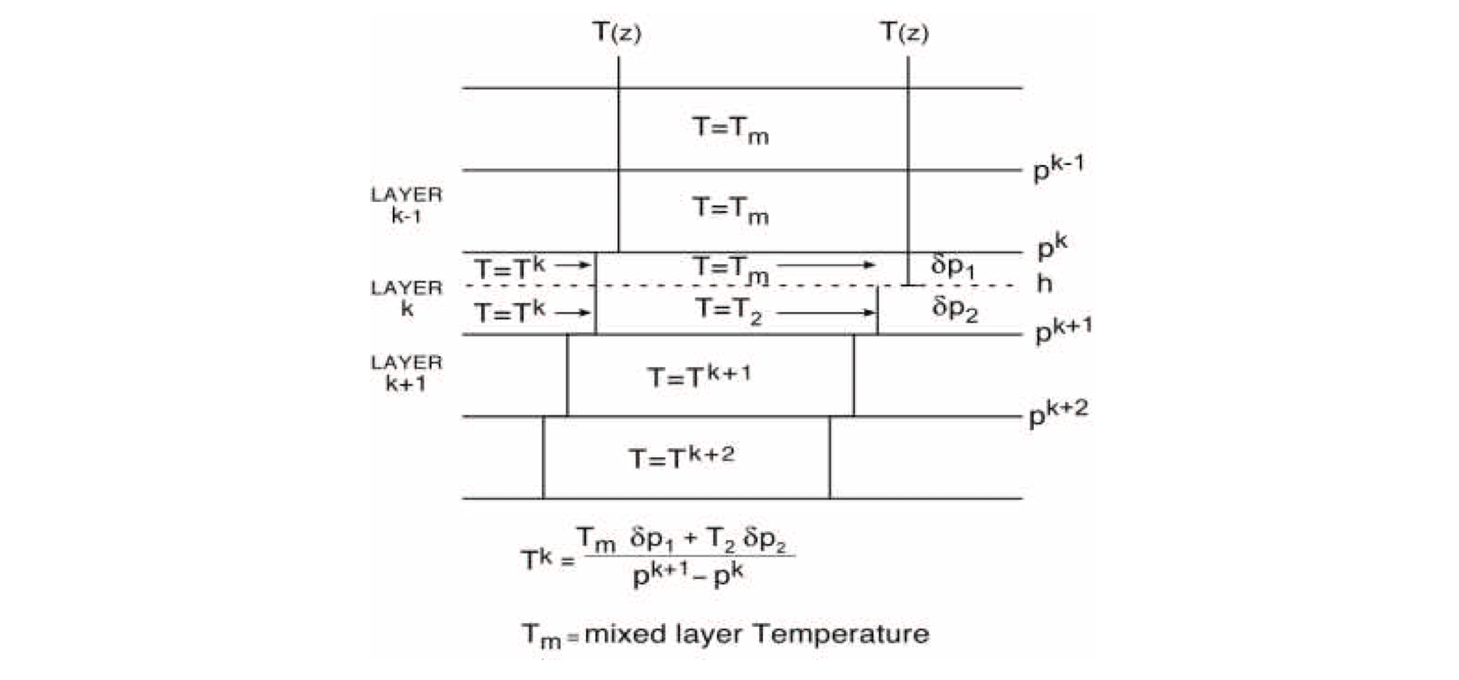
Figure 1. Vertical distribution of a model layer variable (represented by T) in the hybrid KTA slab mixed layer model. The mixed layer base is located at pressure depth h within model layer k. The vertical distribution of T in the HYCOM vertical coordinate system is shown on the left. In the vertical coordinate system used by the KTA model (right) model layer k has been divided into two sublayers above and below the mixed layer base with thicknesses dp₁ and dp₂ to enable the jumps in model variables across the base to be estimated. The value of T in the upper sublayer equals the homogenized mixed layer value. The unmixing algorithm is used to determine the value of T in the lower sublayer (T₂) such that the thickness-weighted vertical average of the sublayer values equals the value of T within HYCOM layer k.