By George Halliwell, 28 November 2004

     The vertical velocity w in Cartesian coordinates is determined by vertically integrating the continuity equation

downward from the surface, where subscripts denote the variable held constant during partial differentiation. Model variables in HYCOM are stored on a non-Cartesian (x,y,s) coordinate system, where the generalized vertical coordinates are surfaces of constant s, typically density in the ocean interior and fixed pressure levels near the ocean surface and in shallow coastal regions. To use equation (1) to estimate w profiles at HYCOM grid points, horizontal velocity components must be re-gridded to constant z levels before integrating (1) downward from the surface. This re-gridding must be performed at high vertical resolution to provide accurate vertical profiles of w.

      Since this high-resolution re-gridding is time consuming, a formula is derived here to estimate w profiles directly from fields stored on the HYCOM generalized coordinate system. This formula is now included in the HYCOM post-processing program (hycomproc) to estimate w profiles from fields stored on model archives. A different formula is then derived to calculate w during HYCOM runs for the purpose of advecting three-dimensional Lagrangian floats. This is accomplished by integrating the HYCOM continuity (thickness tendency) equation downward from the surface and combining it with the previously-derived w profile equation.

      Since HYCOM equations use pressure units for the vertical coordinate, HYCOM vertical velocity is defined as

By converting the vertical coordinate in (1) from z to p , we obtain

Since the HYCOM generalized coordinate system is not Cartesian, integration of (3) downward from the surface introduces additional terms related to the sloping s interfaces. The vertical discretization consists of layers k = 1,2,...,N, with each layer k bounded by vertical coordinate surfaces located at pressure depths p_k(x,y,s) above and p_k+1(x,y,s) below. From this point forward, it is understood that s is held constant in partial differentiation and the subscript s is dropped.
      Assuming w = 0 at the surface, vertical velocity at the base of model layer k = 1 is

where the integration is carried out from the surface down to an infinitesimal distance above interface 2. To obtain the vertical velocity at the top of layer 2, the continuity equation is integrated across interface 2 from p₂^- to p₂⁺:

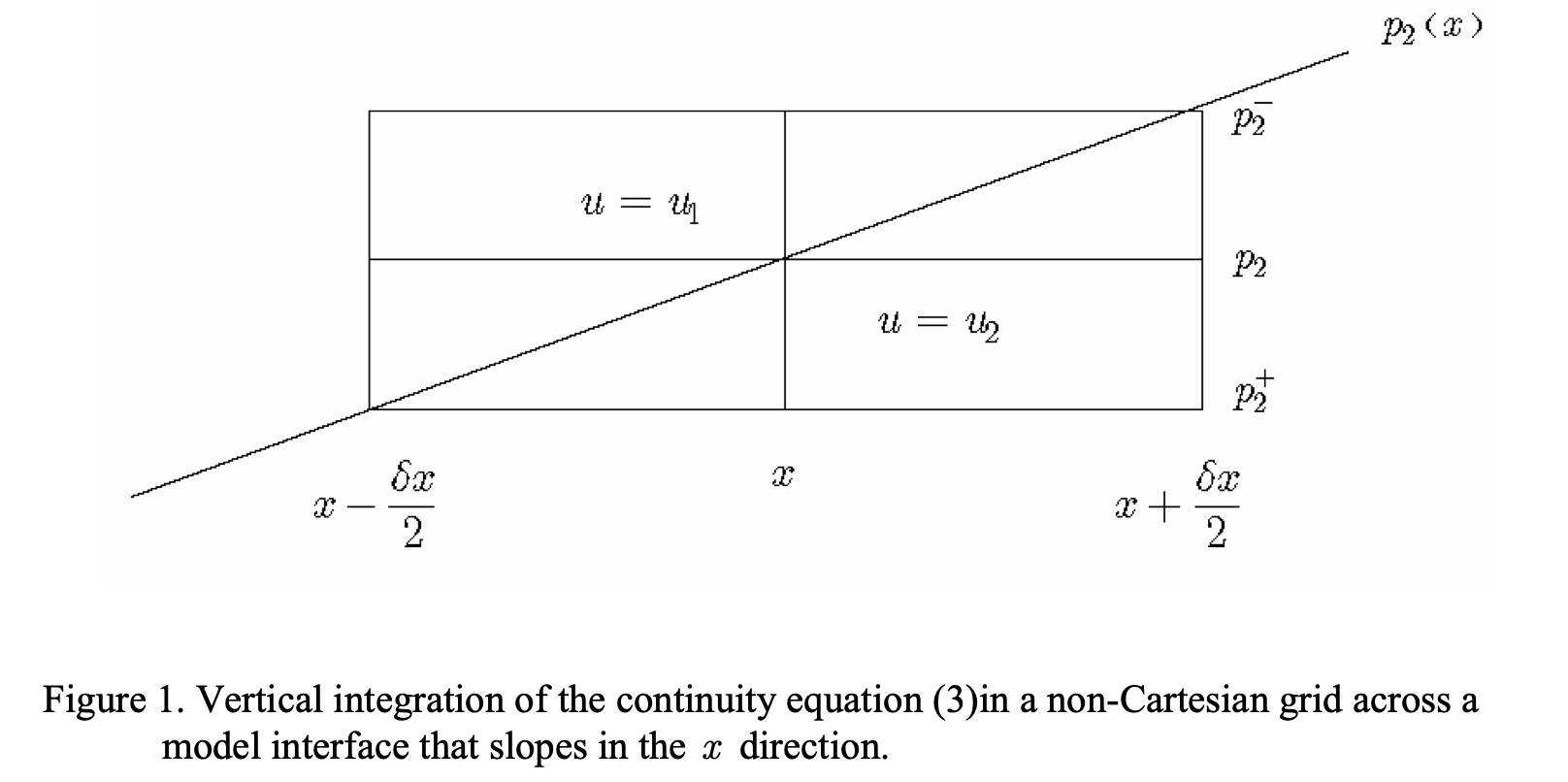
If interface 2 is not level, then a jump condition arises in the evaluation of the rightmost integral in (5). This jump condition is obtained by evaluating the rightmost integral as illustrated for the x direction in Figure 1. The x derivative of u is given by

The vertical velocity jump across the interface is numerically evaluated by

where δp = p₂⁺ - p₂^-. In the limits as the box defined by δx and δp in Figure 1 shrinks to zero area, δp/δx → ∂p/∂x and δx /2 → 0. Thus, w(p₂⁺) from (5) becomes, after adding the jump condition in the y direction

Continuing the integration downward, the vertical velocity at a pressure level P within model layer n ≥ 2, where

is

It is easy to show that

Thus, w varies linearly in the vertical within each layer while discontinuities can exist at model interfaces. Equation (10) is used to evaluate w in the HYCOM post processing program (hycomproc).

      Equation (10) is validated by showing that it gives the correct bottom vertical velocity when integrated from the surface to the bottom. If model layer N is the layer intersecting the bottom (the deepest layer with nonzero thickness), then Equation (10) yields the following expression for vertical velocity at the bottom:

where p_b = p_N +1 is the bottom pressure depth. For this bottom velocity to be correct, it must equal the bottom velocity derived from the continuity equation for the barotropic velocity. Defining barotropic velocity components u,v as vertical averages from the surface to the bottom, and assuming that surface vertical velocity is zero, the following bottom vertical velocity is obtained from the barotropic continuity equation:

The barotropic vertical velocity components are given by

Equation (12) is obtained by substituting (14) into (13), which validates (10).

      It is necessary to estimate w during HYCOM runs for the purpose of vertically advecting synthetic floats. This calculation is made more efficient by taking advantage of calculations already made during model runs, specifically the time evolution of the thickness of model layer k calculated by the HYCOM continuity (thickness tendency) equation. The thickness tendency equation is integrated downward from the surface and combined with equation (10) to derive the expression used to estimate w during HYCOM runs.

      If sub-grid scale processes (thickness diffusion) are neglected, the thickness tendency is given by (Bleck, 2002):

where is the entrainment velocity in pressure per unit time across interface k and the subscripts s indicate that the generalized vertical coordinate is held constant during partial differentiation. Equation (15) is summed downward from the surface assuming that the surface interface is stationary. The vertical motion of interface 2, with the subscript s again dropped, is

Continuing to interface 3,

which results in

Rearranging terms yields

More generally, the vertical motion of interface n + 1 at the base of layer n ≥ 2 is

The interface vertical velocity at pressure depth P within model layer n, with P given by (9), is

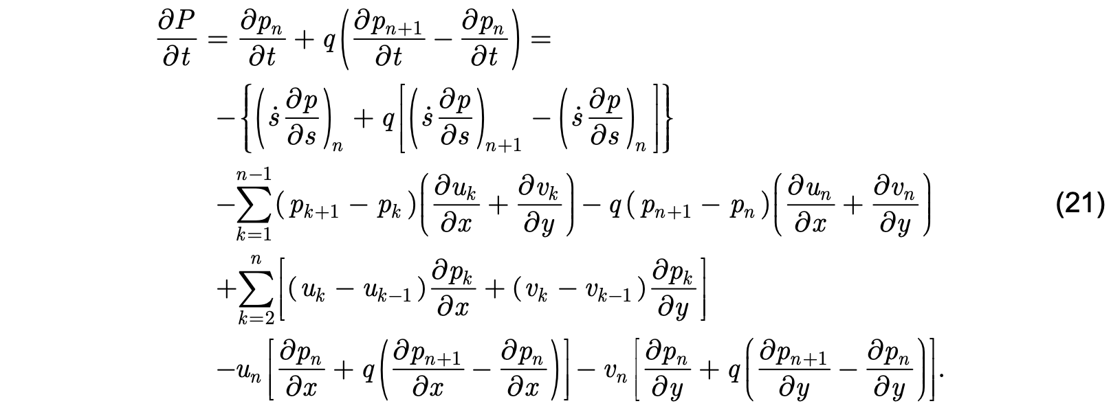
From (10), the third and fourth lines of (21) are identified as the fluid vertical velocity w at pressure depth P. As a result, (21) becomes

The vertical velocity of model pressure interfaces can be separated as follows:

If the entrainment velocity is zero, the interface vertical velocity equals , which can therefore be interpreted as the local vertical velocity of a material surface. Since p_k and p̂_k surfaces are co-located at the time vertical velocity is evaluated, equation (22) can be written as

The first term on the right side of (24) is the vertically interpolated material surface vertical velocity (the vertical velocity of s surfaces in the absence of diapycnal mass fluxes). The other two terms on the right side represent the vertical component of layer k flow when the layer is not flat. It is a function of momentum components within layer n and the slope of the interfaces at the top and bottom of layer n, the latter vertically interpolated to pressure depth P. The vertical velocities at the top and bottom of layer n are obtained by setting q = 0 and q = 1, respectively:

      Vertical velocity at the central depth of layer n is obtained by setting q = 1 / 2:

From Equation (24), the vertical velocity at the ocean bottom reduces to

where p_b is bottom pressure and u_b,v_b are momentum components in the deepest model layer with nonzero thickness.

      To estimate vertical velocities from Equations (24) through (26), it is necessary to estimate at all model interfaces k . It can be obtained by solving the HYCOM thickness diffusion equation (15) with entrainment velocity set to zero:

The advantage to estimating w during model runs is that is already calculated by HYCOM in subroutine cnuity.f. It is only necessary to calculate the interface slope terms and add them to the interface vertical velocity calculated in cnuity.f.

      The two equations for estimating w as a function of pressure P [equations (10) and (24)] are now demonstrated to be equivalent to each other and to w estimated by first re-gridding velocity components onto level pressure coordinates and vertically integrating (3) downward from the surface. Calculations were made within a low-resolution Atlantic simulation. Before integrating (3), horizontal velocity components are re-gridded using

where k_l is the number of the model layer within which pressure depth p is located. The re-gridded velocity components û, v̂ are then substituted into (3). The vertical integration is performed at high vertical resolution (0.1 m, or 0.001 MPa in pressure units) to reduce truncation errors and resolve the velocity jumps that exist across model interfaces. The velocity components are re-gridded onto pressure depths p = 0, 0.001, 0.002, ... MPa and the numerical integration is performed downward from the surface using the trapezoidal rule.

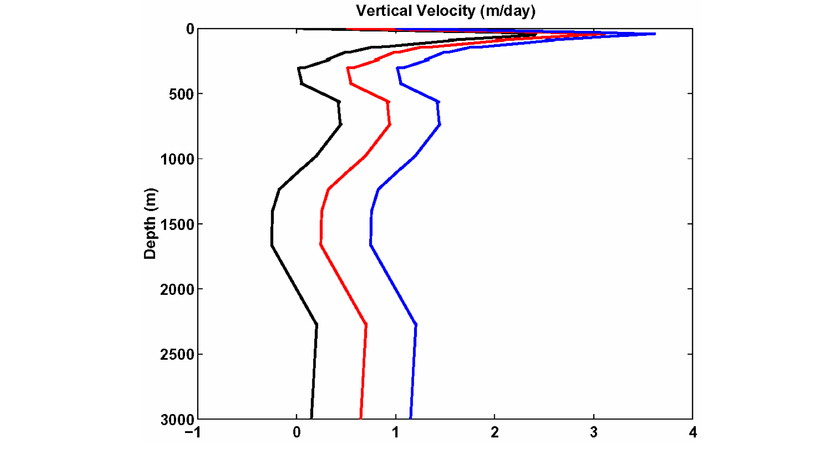
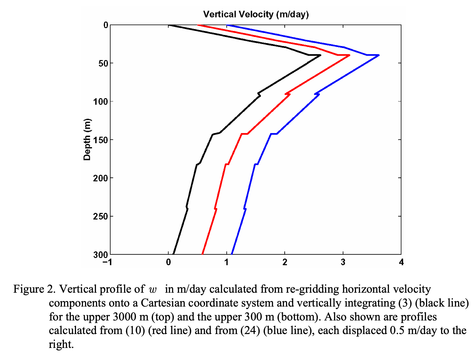
      The w profile resulting from the vertical integration of (3) assuming zero vertical velocity at the surface is illustrated in Figure 2 at the model grid point located on the Equator near 28W. The profiles obtained from equations (10) and (24), varying P in increments of 0.1 m, are also presented in Figure 2. The profiles are identical within numerical truncation errors, validating the derivation of these two equations. Vertical velocity varies linearly within each layer, and jumps can exist across model interfaces. These jumps are most clearly evident in the upper 300 m. The primary difference among the profiles is that the jumps in w occur over a finite depth range in the profiles calculated from (3) because of the horizontal grid spacing (Figure 1). This depth range will decrease toward zero as horizontal grid spacing decreases.

Bleck, R., 2002: An oceanic general circulation model framed in hybrid isopycnic-Cartesian coordinates. Ocean Modelling, 4, 55-88.