UG_Special Topics_Working with R - GoldenCheetah/GoldenCheetah GitHub Wiki
Using the R Chart
The R chart is introduced with v3.4 of GoldenCheetah. The chart can be added to the activity view and the trend view.
Since R is embedded the runtime must match the versions supported by each release of GoldenCheetah
- GC v3.4 supports R < 3.4
- GC v3.5 supports R >= 3.4
When R path is blank GoldenCheetah searches an R install in standard locations, otherwise R path should match the result of R.home() command in R.
Warning: Beware to update your PATH environment variable on Windows after an R version upgrade to avoid errors on R charts. R install must match the architecture of the GC builds, so if you are running GC under Rosetta on Apple Silicon hardware you need to install the an x86-64 version of R.
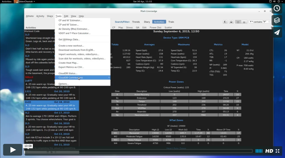
This 10 minute tutorial video introduces the R chart and setup and shows it in use.
In trend view the chart is refreshed when a date range or season is selected, or if the compare pane is updated. Whilst in the activity view the chart is refreshed when an activity is selected or, again, if the compare pane for intervals is updated.
When the chart is refreshed the user supplied R script is executed, and it should collect data and prepare a plot.
A simple example to plot HR might be:
ride <- GC.activity()
plot(ride$heart.rate)
This basically calls a GC function to fetch the data for the current ride and then uses the base R plot function to plot heart rate as a time series.
Similarly, in trend view, to plot a simple time series of average power for the current season:
metrics <- GC.metrics()
plot(metrics$Average_Power)
Local Data, $$ and avoiding data refresh
All data objects are shared across charts. If you create a vector 'x' in one chart it will be available in all the others. Usually, this is not a problem since you fetch the data manipulate it and plot it. But in some cases, where perhaps you prepare data from across the ride data you may want to avoid refreshing it to save time.
If you prefix variable names with $$ then they will get a prefix added to them internally that makes them local to the chart. e.g. $$d internally becomes 'gc0d' on the first chart, 'gc1d' on the second and so on.
We recommend you always prefix variables with $$ to ensure there is not conflict across charts.
If you want to check if a variable exists and already contains values you can use the following code snippet:
> if (!exists("$$p")) print("doesn't exist")
[1] "doesn't exist"
> $$p <- 1
> if (exists("$$p")) print("does exist")
[1] "does exist"
If part of your code prepares large volumes of data, but doesn't need to refresh once its been created then this technique will help speed up your scripts.
Here is an example to get a vector containing all power data across hilly rides, taking care not to repeat on re-run and ignore rides with no power:
## Get one big activity
if (!exists("$$allhills")) {
    $$allhills <- numeric(0)
    for(activity in GC.activity(activity=GC.activities('Workout_Code contains "HILLS"'))) {
        if(length(activity$power) >0 && !anyNA(activity$power))
            $$allhills <- c($$allhills, activity$power)
    }
}
Compare Mode
Where applicable the data access routines will offer a 'compare' parameter to access data; if FALSE it just returns the currently selected ride, if TRUE it will return a list. If compare mode is not active then the list will contain only one set of data for the currently selected ride. If compare is active it returns a list of all things being compared. See GC.activity(compare=TRUE) below for an example.
Search/Filtering
If a search or data filter is active then this will be applied to the results returned by the API methods described below. Even when all=TRUE is set to override season date ranges the filter will be applied. Ultimately, if the user doesn't want a filter to be applied they should clear it. We work this way to ensure consistency across all charts.
Stopping long running scripts
Hitting the ESC key will terminate any long running scripts. This can be useful when processing large volumes of data or an errant script runs into an infinite loop. In general, we would recommend letting long running processes complete, but ESC will terminate them safely.
Contents
Below you will find details of each of the GC functions available to use within the R chart.
- GC.version() to get a version string
- GC.build() to get a build number
- GC.display() to create a new graphics device
- GC.size() to get the window size
- GC.page(width=0, height=0) to set the chart's page size
- GC.athlete() to get the athlete details
- GC.athlete.zones(date=0, sport="") to get zone config
- GC.activities(filter="") to get a list of activities (as dates)
- GC.activity(activity=0,compare=FALSE,split=0,join="repeat") to get the activity data
- GC.activity.metrics(compare=FALSE) to get the activity metrics and metadata
- GC.activity.wbal(compare=FALSE) to get wbal series data
- GC.activity.xdata(name="", compare=FALSE) to get raw xdata series without interpolation
- GC.activity.meanmax(compare=FALSE) to get mean maximals for all activity data
- GC.activity.intervals(type="", activity=0) to get information for the activity intervals
- GC.season(all=FALSE, compare=FALSE) to get season details
- GC.season.metrics(all=FALSE, filter="", compare=FALSE) to get season metrics
- GC.season.meanmax(all=FALSE, filter="", compare=FALSE) to get best mean maximals for a season
- GC.season.peaks(all=FALSE, filter="", compare=FALSE, series, duration) to get activity peaks for a given series and duration
- GC.season.pmc(all=FALSE, metric="TSS") to get PMC data for any given metric
- GC.season.intervals(type="", compare=FALSE) to get metrics for all intervals
- GC.season.measures(all=FALSE, group="Body") to get Daily measures (Body and Hrv available for v3.5)
- GC.setChart(...) to setup chart basics
- GC.addCurve(...) to add a curve to the chart
- GC.setAxis(...) to control axis settings
- GC.annotate(...) to add an annotation to the chart
R Script Examples
Basics
All methods to access and work with GC objects and data within an R chart are prefixed with "GC." this is to ensure there is no namespace clash with other packages you may have installed. There are a number of methods available as listed below.
GC.build() and GC.version()
GC.build will return the build number which increments with each release (including pre-release development builds), you can use this if you need to make a script dependant on the build. Additionally, GC.version will return a string describing the release,which could be put in files or on screen etc.
e.g:
> GC.build()
[1] 3941
> GC.version()
[1] "V4.0 DEV1604"
>
GC.display(), GC.size() and GC.page(width=500, height=500)
If you are familiar with the R device model (dev.cur, dev.list, dev.set) and frequently switch between graphics devices then you can create a new GC graphics device (to plot within the chart) by using GC.display(). If you are not familiar with the R device model then you should probably avoid using this function.
If you want to change the page size used for plotting you can set it with GC.page(). You express the page size in 72 dpi pixels. If you choose a very large size (e.g. 2500x1200) then be sure to have a large screen, since when scaled it will make the fonts very small indeed.
We typically use 500x500, 800x600 and 900x600 for scatter, histogram and time series plots. Be sure to set he page size before any plotting takes place. If you change page size mid-plot you will likely have issues. The command always returns 0.
From v3.5 it is now possible to get the window dimensions (perhaps to decide how to layout the output), the function GC.size() will return a vector with 2 values for width then height.
NOTE: the page size is reset to 500x500 on 3.4, but the window size in all later releases before every script run, so be sure to set it specifically in each plot.
e.g. to set page size to 800x600
> GC.page(width=800, height=600)
integer(0)
>
Athlete
GC.athlete()
GC.athlete() will return a list of athlete details including name, home directory, gender, height, weight and date of birth.
e.g.
> GC.athlete()
$name
[1] "Mark Liversedge"

$home
[1] "/Users/markliversedge/Athletes/Mark Liversedge"

$dob
[1] "1967-07-03"

$weight
[1] 80

$height
[1] 1.83

$gender
[1] "male"

>
GC.athlete.zones(date=0, sport="")
Will return a dataframe of the zone configuration by sport in chronological order. The pace, heartrate and power settings are folded together by sport.
You can specify a date you want to get configuration for, or limit to zone config for a specific sport.
Getting all zone config e.g.
> GC.athlete.zones()
         date sport  cp wprime pmax ftp lthr rhr hrmax cv
1  1900-01-01   run   0      0    0   0  160  57   190 12
2  1900-01-01  bike 250  17000  900 250    0   0     0  0
3  2000-01-01  bike 200  22000  900 200  163  50   188  0
4  2001-01-01  bike 200  22000  900 200  160  57   188  0
5  2007-01-01  bike 275  20000  900 275  160  57   188  0
6  2008-01-01  bike 250  20000  900 250  160  57   188  0
7  2009-01-01  bike 265  20000  900 265  160  57   188  0
8  2009-02-01  bike 275  20000  900 275  160  57   188  0
9  2009-08-01  bike 270  20000  900 270  160  57   188  0
10 2010-01-01  bike 240  20000  900 240  160  57   188  0
11 2010-07-26  bike 180  20000  900 180  160  57   188  0
12 2010-08-11  bike 200  20000  900 200  160  57   188  0
13 2010-09-01  bike 255  22000  900 235  160  57   188  0
14 2012-08-01  bike 220  20000  900 220  160  57   188  0
15 2012-09-08  bike 225  20000  900 225  160  57   188  0
16 2013-04-24  bike 235  20000  900 235  160  57   188  0
17 2013-11-03  bike 250  21000  900 250  160  57   188  0
18 2014-04-01  bike 210  21000  800 210  160  57   188  0
19 2014-11-01  bike 220  22000  800 220  160  57   188  0
20 2015-07-02  bike 220  22000  800 220  165  45   173  0
21 2015-08-01  bike 225  19000  780 250  165  45   173  0
>
And here we get the CP value for the currently selected activity, along the way looking at the values we are using e.g:
> date <- GC.activity.metrics()$date
> date
[1] "2016-05-05"
> GC.athlete.zones(date=date)
        date sport  cp wprime pmax ftp lthr rhr hrmax cv
1 2016-05-05  bike 225  19000  780 250  165  45   173  0
2 2016-05-05   run   0      0    0   0  160  57   190 12
> GC.athlete.zones(date=date, sport="bike")
        date sport  cp wprime pmax ftp lthr rhr hrmax cv
1 2016-05-05  bike 225  19000  780 250  165  45   173  0
> cp <- GC.athlete.zones(date=date, sport="bike")$cp[1]
> cp
[1] 225
>
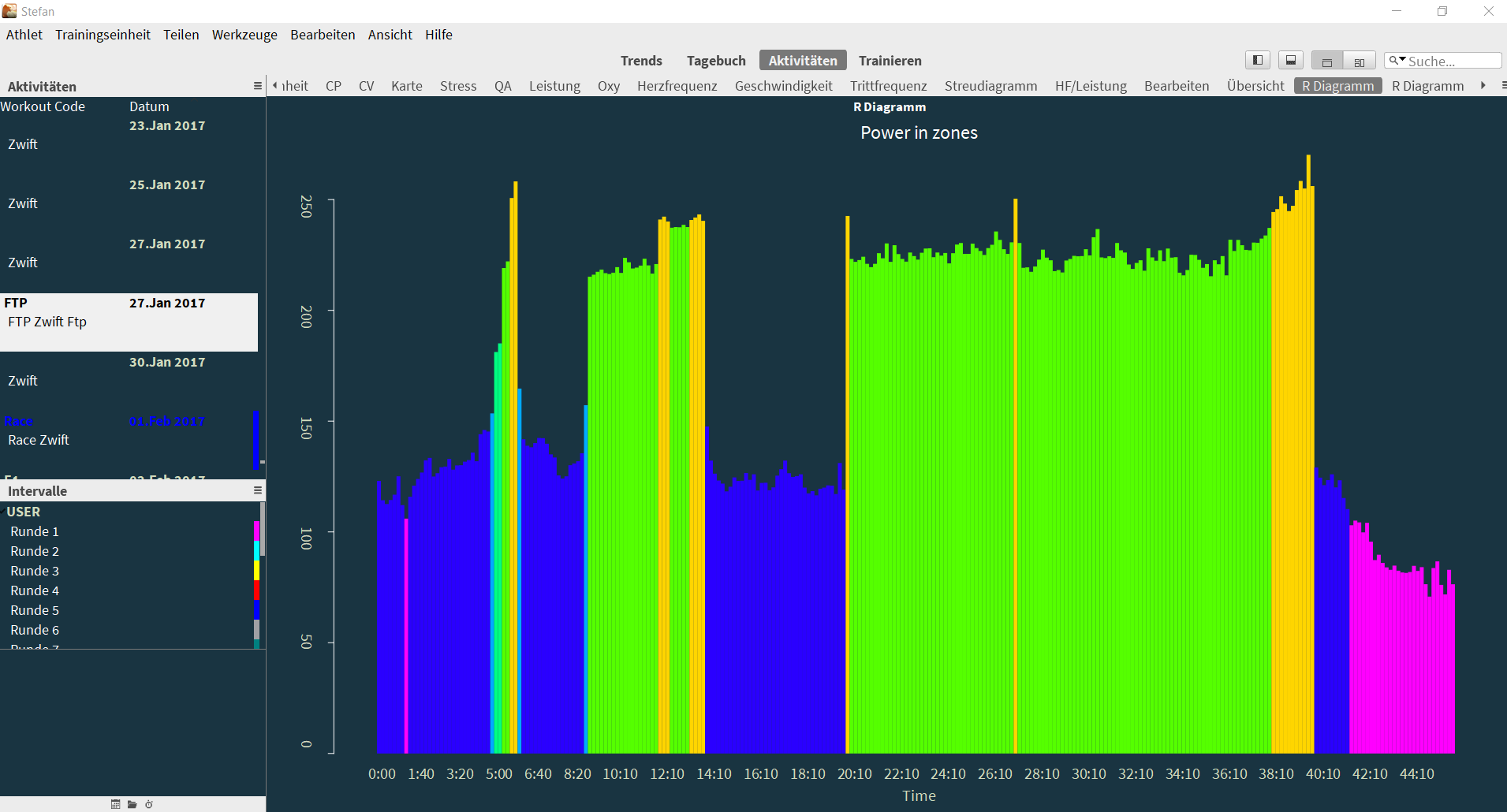
Note: introduced in v3.5 of GoldenCheetah zoneslow and zonescolor, in v3.6 hrzoneslow and pacezoneslow
GC.athlete.zones(date=date, sport="Bike")$zoneslow
GC.athlete.zones(date=date, sport="Bike")$zonescolor
These two properties return lists; zoneslow contains the lower ends of the powerzones and zonescolor the appropriate color hex value.
They can be used to draw charts like this, which shows power in zones over time:
$$activity <- GC.activity()
$$metrics <- GC.metrics()
$$date <- $$metrics$date

$$zone <- GC.athlete.zones(date=$$date, sport="Bike")
$$lows <- $$zone$zoneslow
$$colors <- $$zone$zonescolor

$$duration <- tail($$activity$seconds, n=1)
$$p <- $$activity$power

$$n = 10
$$group <- split($$p, ceiling(seq_along($$p)/$$n))
$$p2 <- sapply($$group, mean)

$$time <- $$activity$seconds[seq(1, length($$activity$seconds), $$n)]
$$breaks <- c(unlist($$lows), Inf)
$$cols <- c(unlist($$colors))[findInterval($$p2, vec=$$breaks)]

$$displaytime <- function(timevalue) {
	$$totalMinutes <- timevalue %/% 60
	$$totalSeconds <- sprintf("%02d", timevalue %% 60)
 	paste($$totalMinutes, $$totalSeconds, sep=":")
}

barplot($$p2,
	names.arg=lapply($$time, $$displaytime),
	space=0, border=NA,
	col=$$cols
)
title(main="Power in zones", ylab = "Watts", xlab = "Time")
Activity
In the activity view you will work primarily with activities. The functions listed below return data related to the currently selected activity or are directly related to that context.
GC.activities(filter="")
Will return a vector of POSIXct datetimes representing the start time for each activity. As the API matures it is expected that you will be able to reference a specific athletes activity via its start time.
e.g.
> d <- GC.activities()
> str(d)
 POSIXct[1:705], format: "2005-06-25 14:26:00" "2005-06-27 08:39:00" ...
>
The filter parameter will be applied as a datafilter to limit the results, enabling you to select specific types of rides. You can pass multiple filters as a string vector.
e.g.
> l <- GC.activities(filter='Workout_Code="1L2"')
> str(l)
 POSIXct[1:65], format: "2008-12-29 12:33:49" "2009-02-12 12:00:00" ...
>
GC.activity(activity=0, compare=FALSE, split=0, join="repeat")
By default (compare=FALSE) it will return a data.frame representing the data for the currently selected ride. The column names have been selected to remain compatible with the trackeR package from UCL for analysing GPS based sports data.
The data.frame returned looks like this when using the 'str' command:
R Console (3.3.0)
> df <- GC.activity()
> str(df)
'data.frame':	3713 obs. of  21 variables:
 $ time        : POSIXct, format: "2016-05-04 15:00:19" "2016-05-04 15:00:20" ...
 $ seconds     : num  0 1 2 3 4 5 6 7 8 9 ...
 $ cadence     : num  0 0 0 0 0 0 0 0 0 0 ...
 $ cadenced    : num  0 0 0 0 0 0 0 0 0 0 ...
 $ heart.rate  : num  NA NA NA NA NA NA NA NA NA NA ...
 $ heart.rated : num  NA NA NA NA NA NA NA NA NA NA ...
 $ distance    : num  0 0 0 0 0 0 0 0 0 0 ...
 $ speed       : num  5.1 5.1 5.38 5.65 5.93 ...
 $ acceleration: num  0 0 0.0772 0.0772 0.0772 ...
 $ torque      : num  NA NA NA NA NA NA NA NA NA NA ...
 $ torqued     : num  NA NA NA NA NA NA NA NA NA NA ...
 $ power       : num  0 0 0 0 0 0 0 0 0 0 ...
 $ powerd      : num  0 0 0 0 0 0 0 0 0 0 ...
 $ altitude    : num  66 66 66 66 66 66 66 66 66 66 ...
 $ longitude   : num  -0.479 -0.479 -0.479 -0.479 -0.479 ...
 $ latitude    : num  51.1 51.1 51.1 51.1 51.1 ...
 $ headwind    : num  5.1 5.1 5.38 5.65 5.93 ...
 $ slope       : num  0 0 0 0 0 0 0 0 0 0 ...
 $ temperature : num  27 27 27 27 27 27 27 27 27 27 ...
 $ apower      : num  0 0 0 0 0 0 0 0 0 0 ...
 $ gearratio   : num  0 0 0 0 0 0 0 0 0 0 ...
>
Depending upon the data you have available in the activity you may see more columns, for example pedal based power meters and muscle oxygen devices will return additional data. In this example above you will see that heartrate and torque data is not recorded but still present in the data.frame -- the columns listed above will always be made available but will contan R's NA value if not actually recorded in the activity.
GC.activity(split=n)
You can specify the minimum gap that will cause the activity returned to be split into separate activities (as a list). split is passed in seconds, where a value of 0 (the default) will disable splitting.
GC.activity(join="repeat")
When an activity contains XDATA (extensible data) then all the xdata series are returned with the standard sample data. The join can be specified, it defaults to repeat, but can be one of:
- repeat - if no value is present for a given point in time, repeat the last value seen
- interpolate - interpolate values where they are missing
- sparse - only return a value when there is one present in the xdata series
- resample - for now, same as interpolate, but we may extend to down/up sample data to a new sampling rate.
Here is an example of an activity with rowing xdata:
> str(GC.activity())
'data.frame':	220 obs. of  42 variables:
 $ time                 : POSIXct, format: "2016-07-19 15:56:09" "2016-07-19 15:56:11" ...
 $ seconds              : num  0 2.02 4.45 6.85 9.18 ...
 $ cadence              : num  NA NA NA NA NA NA NA NA NA NA ...
 $ cadenced             : num  NA NA NA NA NA NA NA NA NA NA ...
 $ heart.rate           : num  0 0 0 0 0 0 0 0 0 0 ...
 $ heart.rated          : num  0 0 0 0 0 0 0 0 0 0 ...
 $ distance             : num  0 0.00306 0.0072 0.0118 0.01662 ...
 $ speed                : num  NA NA NA NA NA NA NA NA NA NA ...
 $ acceleration         : num  NA NA NA NA NA NA NA NA NA NA ...
 $ torque               : num  NA NA NA NA NA NA NA NA NA NA ...
 $ torqued              : num  NA NA NA NA NA NA NA NA NA NA ...
 $ power                : num  7.01 12.96 20.18 26.36 32.51 ...
 $ powerd               : num  0 2.95 2.97 2.58 2.64 ...
 $ altitude             : num  NA NA NA NA NA NA NA NA NA NA ...
 $ longitude            : num  NA NA NA NA NA NA NA NA NA NA ...
 $ latitude             : num  NA NA NA NA NA NA NA NA NA NA ...
 $ headwind             : num  NA NA NA NA NA NA NA NA NA NA ...
 $ ROW_ID               : num  28920100 28920100 28920100 28920100 28920100 ...
 $ ROW_INTERVAL         : num  260891 260891 260891 260891 260891 ...
 $ ROW_REF              : num  21895 21896 21897 21898 21899 ...
 $ ROW_STROKE           : num  1 2 3 4 5 6 7 8 9 10 ...
 $ ROW_POWER            : num  7.01 12.96 20.18 26.36 32.51 ...
 $ ROW_AVGPOWER         : num  7.01 9.98 13.38 16.62 19.8 ...
 $ ROW_STROKERATE       : num  47.5 29 24.3 24.7 25.2 ...
 $ ROW_TIME             : num  1.26 3.28 5.71 8.11 10.44 ...
 $ ROW_STROKELENGTH     : num  72.6 61.6 77 77 79.2 74.8 77 74.8 72.6 72.6 ...
 $ ROW_DISTANCE         : num  1.55 4.61 8.75 13.35 18.17 ...
 $ ROW_STROKEDISTANCE   : num  155 306 413 461 482 ...
 $ ROW_ESTIMATE500MTIME : num  408 337 298 264 247 ...
 $ ROW_STROKEENERGY     : num  155.5 83.2 119.8 114.3 132.3 ...
 $ ROW_ENERGYSUM        : num  0.16 0.24 0.36 0.47 0.61 0.73 0.86 0.98 1.11 1.23 ...
 $ ROW_PULSE            : num  0 0 0 0 0 0 0 0 0 0 ...
 $ ROW_WORKPERPULSE     : num  0 0 0 0 0 0 0 0 0 0 ...
 $ ROW_PEAKFORCE        : num  123 110 130 117 137 131 129 132 132 132 ...
 $ ROW_PEAKFORCEPOS     : num  15.4 26.4 28.6 30.8 35.2 24.2 30.8 26.4 33 26.4 ...
 $ ROW_PEAKFORCERELPOS  : num  21.2 42.9 37.1 40 44.4 ...
 $ ROW_DRIVETIME        : num  1.26 0.84 0.91 0.83 0.79 0.71 0.71 0.68 0.65 0.64 ...
 $ ROW_RECOVERTIME      : num  0 1.23 1.56 1.6 1.59 1.61 1.63 1.64 1.59 1.59 ...
 $ ROW_K                : num  0.1 0.09 0.09 0.09 0.09 0.09 0.09 0.09 0.09 0.09 ...
 $ ROW_CURVEDATA        : num  0 0 0 0 0 0 0 0 0 0 ...
 $ ROW_STROKENUMINTERVAL: num  1 2 3 4 5 6 7 8 9 10 ...
 $ ROW_AVGPOWER         : num  7.01 9.98 13.38 16.62 19.8 ...
>
GC.activity(compare=TRUE)
If you pass the parameter compare=TRUE then the format returned is a list rather than a dataframe. The lis contains an entry for each ride being compared, or just the currently selected ride if compare is not active.
Each entry in the list contains two elements; 'color' a string you can use in 'col="xxx"' assignments, and 'activity' the data.frame in the same format as above.
e.g. with compare not active:
> df <- GC.activity(compare=TRUE)
> str(df)
Dotted pair list of 1
 $ :Dotted pair list of 2
  ..$ activity:'data.frame':	3713 obs. of  21 variables:
  .. ..$ time        : POSIXct[1:3713], format: "2016-05-04 15:00:19" "2016-05-04 15:00:20" ...
  .. ..$ seconds     : num [1:3713] 0 1 2 3 4 5 6 7 8 9 ...
  .. ..$ cadence     : num [1:3713] 0 0 0 0 0 0 0 0 0 0 ...
  .. ..$ cadenced    : num [1:3713] 0 0 0 0 0 0 0 0 0 0 ...
  .. ..$ heart.rate  : num [1:3713] NA NA NA NA NA NA NA NA NA NA ...
  .. ..$ heart.rated : num [1:3713] NA NA NA NA NA NA NA NA NA NA ...
  .. ..$ distance    : num [1:3713] 0 0 0 0 0 0 0 0 0 0 ...
  .. ..$ speed       : num [1:3713] 5.1 5.1 5.38 5.65 5.93 ...
  .. ..$ acceleration: num [1:3713] 0 0 0.0772 0.0772 0.0772 ...
  .. ..$ torque      : num [1:3713] NA NA NA NA NA NA NA NA NA NA ...
  .. ..$ torqued     : num [1:3713] NA NA NA NA NA NA NA NA NA NA ...
  .. ..$ power       : num [1:3713] 0 0 0 0 0 0 0 0 0 0 ...
  .. ..$ powerd      : num [1:3713] 0 0 0 0 0 0 0 0 0 0 ...
  .. ..$ altitude    : num [1:3713] 66 66 66 66 66 66 66 66 66 66 ...
  .. ..$ longitude   : num [1:3713] -0.479 -0.479 -0.479 -0.479 -0.479 ...
  .. ..$ latitude    : num [1:3713] 51.1 51.1 51.1 51.1 51.1 ...
  .. ..$ headwind    : num [1:3713] 5.1 5.1 5.38 5.65 5.93 ...
  .. ..$ slope       : num [1:3713] 0 0 0 0 0 0 0 0 0 0 ...
  .. ..$ temperature : num [1:3713] 27 27 27 27 27 27 27 27 27 27 ...
  .. ..$ apower      : num [1:3713] 0 0 0 0 0 0 0 0 0 0 ...
  .. ..$ gearratio   : num [1:3713] 0 0 0 0 0 0 0 0 0 0 ...
  ..$ color   : chr "#FF00FF"
>
e.g. with compare active and two rides in the compare pane:
> df <- GC.activity(compare=TRUE)
> str(df)
Dotted pair list of 2
 $ :Dotted pair list of 2
  ..$ activity:'data.frame':	3712 obs. of  21 variables:
  .. ..$ time        : POSIXct[1:3712], format: "2016-05-04 15:00:19" "2016-05-04 15:00:20" ...
  .. ..$ seconds     : num [1:3712] 0 1 2 3 4 5 6 7 8 9 ...
  .. ..$ cadence     : num [1:3712] 0 0 0 0 0 0 0 0 0 0 ...
  .. ..$ cadenced    : num [1:3712] 0 0 0 0 0 0 0 0 0 0 ...
  .. ..$ heart.rate  : num [1:3712] NA NA NA NA NA NA NA NA NA NA ...
  .. ..$ heart.rated : num [1:3712] NA NA NA NA NA NA NA NA NA NA ...
  .. ..$ distance    : num [1:3712] 0 0 0 0 0 0 0 0 0 0 ...
  .. ..$ speed       : num [1:3712] 5.1 5.1 5.38 5.65 5.93 ...
  .. ..$ acceleration: num [1:3712] 0 0 0.0772 0.0772 0.0772 ...
  .. ..$ torque      : num [1:3712] NA NA NA NA NA NA NA NA NA NA ...
  .. ..$ torqued     : num [1:3712] NA NA NA NA NA NA NA NA NA NA ...
  .. ..$ power       : num [1:3712] 0 0 0 0 0 0 0 0 0 0 ...
  .. ..$ powerd      : num [1:3712] 0 0 0 0 0 0 0 0 0 0 ...
  .. ..$ altitude    : num [1:3712] 66 66 66 66 66 66 66 66 66 66 ...
  .. ..$ longitude   : num [1:3712] -0.479 -0.479 -0.479 -0.479 -0.479 ...
  .. ..$ latitude    : num [1:3712] 51.1 51.1 51.1 51.1 51.1 ...
  .. ..$ headwind    : num [1:3712] 5.1 5.1 5.38 5.65 5.93 ...
  .. ..$ slope       : num [1:3712] 0 0 0 0 0 0 0 0 0 0 ...
  .. ..$ temperature : num [1:3712] 27 27 27 27 27 27 27 27 27 27 ...
  .. ..$ apower      : num [1:3712] 0 0 0 0 0 0 0 0 0 0 ...
  .. ..$ gearratio   : num [1:3712] 0 0 0 0 0 0 0 0 0 0 ...
  ..$ color   : chr "#ff00ff"
 $ :Dotted pair list of 2
  ..$ activity:'data.frame':	4534 obs. of  21 variables:
  .. ..$ time        : POSIXct[1:4534], format: "2016-05-03 14:45:57" "2016-05-03 14:45:58" ...
  .. ..$ seconds     : num [1:4534] 0 1 2 3 4 5 6 7 8 9 ...
  .. ..$ cadence     : num [1:4534] 78 71 72 133 133 133 60 93 93 93 ...
  .. ..$ cadenced    : num [1:4534] 0 0 1 61 0 0 0 33 0 0 ...
  .. ..$ heart.rate  : num [1:4534] NA NA NA NA NA NA NA NA NA NA ...
  .. ..$ heart.rated : num [1:4534] NA NA NA NA NA NA NA NA NA NA ...
  .. ..$ distance    : num [1:4534] 0 0.006 0.012 0.012 0.012 0.014 0.02 0.02 0.02 0.02 ...
  .. ..$ speed       : num [1:4534] 0 24.8 30.7 30.7 30.7 ...
  .. ..$ acceleration: num [1:4534] 0 6.89 1.64 0 0 ...
  .. ..$ torque      : num [1:4534] NA NA NA NA NA NA NA NA NA NA ...
  .. ..$ torqued     : num [1:4534] NA NA NA NA NA NA NA NA NA NA ...
  .. ..$ power       : num [1:4534] 0 34 20 0 0 0 11 11 11 11 ...
  .. ..$ powerd      : num [1:4534] 0 34 0 0 0 0 11 0 0 0 ...
  .. ..$ altitude    : num [1:4534] -33 -32 -32 -32 -32 -32 -32 -32 -32 -32 ...
  .. ..$ longitude   : num [1:4534] NA NA NA NA NA NA NA NA NA NA ...
  .. ..$ latitude    : num [1:4534] NA NA NA NA NA NA NA NA NA NA ...
  .. ..$ headwind    : num [1:4534] 0 24.8 30.7 30.7 30.7 ...
  .. ..$ slope       : num [1:4534] 0 16.7 0 0 0 ...
  .. ..$ temperature : num [1:4534] 17 18 18 18 18 18 18 18 18 18 ...
  .. ..$ apower      : num [1:4534] 0 34 20 0 0 0 11 11 11 11 ...
  .. ..$ gearratio   : num [1:4534] 0 2.7 3 3 3 3 3.5 2.3 2.3 2.3 ...
  ..$ color   : chr "#00ffff"
>
In this way, if you want to remain compatible with compare mode when charting you should always use 'compare=TRUE' and loop through the results to plot, taking care to overplot using 'lines', 'points' or 'curve'.
You can specify the activity (or activities) you want to fetch by using the parameter activity. It should be set to a POSIXct datetime, or a vector. Remember that GC.activities() will return a vector of POSIXct representing each activity.
The example below retrieves raw sample data, in a dataframe for 13 rides where the 'Test' metadata flag is non-zero, e.g:
> list <- GC.activities(filter="Test <> 0")
> list
 [1] "2007-04-13 10:00:00 UTC" "2008-12-03 11:31:32 UTC"
 [3] "2009-01-24 15:11:21 UTC" "2009-02-07 11:38:22 UTC"
 [5] "2009-02-13 14:05:37 UTC" "2009-02-26 11:31:16 UTC"
 [7] "2009-03-09 12:35:23 UTC" "2009-04-20 10:33:16 UTC"
 [9] "2009-05-13 18:18:39 UTC" "2010-08-07 11:34:20 UTC"
[11] "2010-09-22 16:11:33 UTC" "2012-05-28 18:04:02 UTC"
[13] "2015-10-22 15:57:58 UTC"
> rides <- GC.activity(activity=list)
> str(rides)
Dotted pair list of 13
 $ 1 :'data.frame':	2817 obs. of  18 variables:
  ..$ time        : POSIXct[1:2817], format: "2007-04-13 10:00:00" "2007-04-13 10:00:01" ...
  ..$ seconds     : num [1:2817] 0 1.26 2.52 3.78 5.04 ...
  ..$ cadence     : num [1:2817] 93 93 59 99 103 76 76 76 93 93 ...
  ..$ cadenced    : num [1:2817] 0 0 0 31.75 3.17 ...
  ..$ heart.rate  : num [1:2817] NA NA NA NA NA NA NA NA NA NA ...
  ..$ heart.rated : num [1:2817] NA NA NA NA NA NA NA NA NA NA ...
  ..$ distance    : num [1:2817] 0 0.013 0.027 0.044 0.059 0.074 0.088 0.103 0.118 0.13 ...
  ..$ speed       : num [1:2817] 39.9 39.9 42.3 43.5 43.6 43.5 43.5 43.5 42.1 41.5 ...
  ..$ acceleration: num [1:2817] 0 0 0.529 0.265 0.022 ...
  ..$ torque      : num [1:2817] 5.2 5.2 5.6 5 5.4 6.9 6.9 6.9 8.9 8.5 ...
  ..$ torqued     : num [1:2817] 0 0 0.317 -0.476 0.317 ...
  ..$ power       : num [1:2817] 173 173 199 180 197 249 249 249 313 293 ...
  ..$ powerd      : num [1:2817] 0 0 20.6 0 13.5 ...
  ..$ altitude    : num [1:2817] NA NA NA NA NA NA NA NA NA NA ...
  ..$ longitude   : num [1:2817] NA NA NA NA NA NA NA NA NA NA ...
  ..$ latitude    : num [1:2817] NA NA NA NA NA NA NA NA NA NA ...
  ..$ headwind    : num [1:2817] NA NA NA NA NA NA NA NA NA NA ...
  ..$ gearratio   : num [1:2817] 3 3 3 3 3 4.5 4.5 4.5 3.5 3.5 ...
 $ 2 :'data.frame':	4029 obs. of  18 variables:
  ..$ time        : POSIXct[1:4029], format: "2008-12-03 11:31:32" "2008-12-03 11:31:33" ...
  ..$ seconds     : num [1:4029] 0 1.26 2.52 3.78 5.04 ...
  ..$ cadence     : num [1:4029] 0 0 0 0 0 0 0 0 0 0 ...
  ..$ cadenced    : num [1:4029] 0 0 0 0 0 0 0 0 0 0 ...
  ..$ heart.rate  : num [1:4029] 78 80 82 83 85 84 83 83 81 81 ...
  ..$ heart.rated : num [1:4029] 0 1.587 1.587 0.794 1.587 ...
  ..$ distance    : num [1:4029] 0 0 0 0.002 0.002 0.002 0.002 0.002 0.002 0.004 ...
  ..$ speed       : num [1:4029] 0 0 0 0 0 0 0 0 0 0 ...
  ..$ acceleration: num [1:4029] 0 0 0 0 0 0 0 0 0 0 ...
  ..$ torque      : num [1:4029] 0 0 0 0 0 0 0 0 0 0 ...
  ..$ torqued     : num [1:4029] 0 0 0 0 0 0 0 0 0 0 ...
  ..$ power       : num [1:4029] 0 0 0 0 0 0 0 0 0 0 ...
  ..$ powerd      : num [1:4029] 0 0 0 0 0 0 0 0 0 0 ...
  ..$ altitude    : num [1:4029] NA NA NA NA NA NA NA NA NA NA ...
  ..$ longitude   : num [1:4029] NA NA NA NA NA NA NA NA NA NA ...
  ..$ latitude    : num [1:4029] NA NA NA NA NA NA NA NA NA NA ...
  ..$ headwind    : num [1:4029] NA NA NA NA NA NA NA NA NA NA ...
  ..$ gearratio   : num [1:4029] 0 0 0 0 0 0 0 0 0 0 ...
 $ 3 :'data.frame':	4523 obs. of  20 variables:
  ..$ time        : POSIXct[1:4523], format: "2009-01-24 15:11:21" "2009-01-24 15:11:22" ...
  ..$ seconds     : num [1:4523] 0 1 2 5 6 7 8 9 10 11 ...
  ..$ cadence     : num [1:4523] 0 0 0 0 2 2 16 38 51 60 ...
  ..$ cadenced    : num [1:4523] 0 0 0 0 2 0 14 22 13 9 ...
  ..$ heart.rate  : num [1:4523] 75 75 74 75 75 75 77 80 81 86 ...
  ..$ heart.rated : num [1:4523] 0 0 -1 0.333 0 ...
  ..$ distance    : num [1:4523] 0 0 0.004 0.004 0.006 0.01 0.014 0.021 0.027 0.032 ...
  ..$ speed       : num [1:4523] 0 0.5 4.3 2.6 6.3 14 15.6 21.9 22.9 19.7 ...
  ..$ acceleration: num [1:4523] 0 0.139 1.056 -0.157 1.028 ...
  ..$ torque      : num [1:4523] NA NA NA NA NA NA NA NA NA NA ...
  ..$ torqued     : num [1:4523] NA NA NA NA NA NA NA NA NA NA ...
  ..$ power       : num [1:4523] 0 0 0 0 0 0 329 500 477 561 ...
  ..$ powerd      : num [1:4523] 0 0 0 0 0 0 329 171 0 84 ...
  ..$ altitude    : num [1:4523] 166 166 166 166 166 ...
  ..$ longitude   : num [1:4523] -0.479 -0.479 -0.479 -0.479 -0.479 ...
  ..$ latitude    : num [1:4523] 51.1 51.1 51.1 51.1 51.1 ...
  ..$ headwind    : num [1:4523] NA NA NA NA NA NA NA NA NA NA ...
  ..$ slope       : num [1:4523] 0 0 -2.5 0 0 ...
  ..$ apower      : num [1:4523] 0 0 0 0 0 ...
  ..$ gearratio   : num [1:4523] 0 0 0 0 0 0 0 3.5 3.5 2.6 ...
 $ 4 :'data.frame':	4279 obs. of  20 variables:
  ..$ time        : POSIXct[1:4279], format: "2009-02-07 11:38:22" "2009-02-07 11:38:23" ...
  ..$ seconds     : num [1:4279] 0 1 2 3 4 5 6 7 8 9 ...
  ..$ cadence     : num [1:4279] 0 0 0 0 0 0 0 4 16 34 ...
  ..$ cadenced    : num [1:4279] 0 0 0 0 0 0 0 4 12 18 ...
  ..$ heart.rate  : num [1:4279] 90 91 93 92 92 95 93 96 97 96 ...
  ..$ heart.rated : num [1:4279] 0 1 2 -1 0 3 -2 3 1 -1 ...
  ..$ distance    : num [1:4279] 0 0 0 0.002 0.003 0.005 0.007 0.011 0.016 0.022 ...
  ..$ speed       : num [1:4279] 0 0.2 0.6 5.6 3.6 7.1 8.6 13.4 17.5 21.7 ...
  ..$ acceleration: num [1:4279] 0 0.0556 0.1111 1.3889 -0.5556 ...
  ..$ torque      : num [1:4279] NA NA NA NA NA NA NA NA NA NA ...
  ..$ torqued     : num [1:4279] NA NA NA NA NA NA NA NA NA NA ...
  ..$ power       : num [1:4279] 0 0 0 0 15 15 15 246 473 551 ...
  ..$ powerd      : num [1:4279] 0 0 0 0 15 0 0 231 227 78 ...
  ..$ altitude    : num [1:4279] 142 142 142 141 141 ...
  ..$ longitude   : num [1:4279] -0.479 -0.479 -0.479 -0.479 -0.479 ...
  ..$ latitude    : num [1:4279] 51.1 51.1 51.1 51.1 51.1 ...
  ..$ headwind    : num [1:4279] NA NA NA NA NA NA NA NA NA NA ...
  ..$ slope       : num [1:4279] 0 0 0 -5 -10 5 -15 5 -6 0 ...
  ..$ apower      : num [1:4279] 0 0 0 0 15.1 ...
  ..$ gearratio   : num [1:4279] 0 0 0 0 0 0 0 0 0 5 ...
 $ 5 :'data.frame':	4020 obs. of  20 variables:
  ..$ time        : POSIXct[1:4020], format: "2009-02-13 14:05:37" "2009-02-13 14:05:38" ...
  ..$ seconds     : num [1:4020] 0 1 2 5 6 7 8 9 10 11 ...
  ..$ cadence     : num [1:4020] 14 0 5 5 19 35 35 46 46 52 ...
  ..$ cadenced    : num [1:4020] 0 0 5 0 14 16 0 11 0 6 ...
  ..$ heart.rate  : num [1:4020] 67 67 67 69 68 68 70 71 74 78 ...
  ..$ heart.rated : num [1:4020] 0 0 0 0.667 -1 ...
  ..$ distance    : num [1:4020] 0 0 0.007 0.009 0.013 0.017 0.023 0.029 0.036 0.043 ...
  ..$ speed       : num [1:4020] 0 0 7.8 7.9 14.3 17.3 19.9 21.3 24.1 26 ...
  ..$ acceleration: num [1:4020] 0 0 2.16667 0.00926 1.77778 ...
  ..$ torque      : num [1:4020] NA NA NA NA NA NA NA NA NA NA ...
  ..$ torqued     : num [1:4020] NA NA NA NA NA NA NA NA NA NA ...
  ..$ power       : num [1:4020] 2 0 6 6 266 370 370 308 407 477 ...
  ..$ powerd      : num [1:4020] 0 0 6 0 260 104 0 0 99 70 ...
  ..$ altitude    : num [1:4020] -24.1 -24.1 -24.1 -24.5 -24.7 -24.8 -24.3 -24.6 -24.4 -24.6 ...
  ..$ longitude   : num [1:4020] -0.479 -0.479 -0.479 -0.479 -0.479 ...
  ..$ latitude    : num [1:4020] 51.1 51.1 51.1 51.1 51.1 ...
  ..$ headwind    : num [1:4020] NA NA NA NA NA NA NA NA NA NA ...
  ..$ slope       : num [1:4020] 0 0 0 -20 -5 ...
  ..$ apower      : num [1:4020] 2 0 6 6 266 370 370 308 407 477 ...
  ..$ gearratio   : num [1:4020] 0 0 0 0 3.5 3.5 3.5 3.5 3.5 3.5 ...
 $ 6 :'data.frame':	3840 obs. of  20 variables:
  ..$ time        : POSIXct[1:3840], format: "2009-02-26 11:31:16" "2009-02-26 11:31:17" ...
  ..$ seconds     : num [1:3840] 0 1 2 3 4 5 6 7 8 9 ...
  ..$ cadence     : num [1:3840] 0 0 0 0 0 0 0 9 9 49 ...
  ..$ cadenced    : num [1:3840] 0 0 0 0 0 0 0 9 0 40 ...
  ..$ heart.rate  : num [1:3840] 63 63 63 63 64 64 65 66 69 71 ...
  ..$ heart.rated : num [1:3840] 0 0 0 0 1 0 1 1 3 2 ...
  ..$ distance    : num [1:3840] 0 0.001 0.001 0.002 0.004 0.006 0.009 0.014 0.02 0.027 ...
  ..$ speed       : num [1:3840] 0 2.1 2.2 3.5 5.7 7.3 13.1 17.6 20.6 23.5 ...
  ..$ acceleration: num [1:3840] 0 0.5833 0.0278 0.3611 0.6111 ...
  ..$ torque      : num [1:3840] NA NA NA NA NA NA NA NA NA NA ...
  ..$ torqued     : num [1:3840] NA NA NA NA NA NA NA NA NA NA ...
  ..$ power       : num [1:3840] 0 0 0 0 0 0 0 482 482 563 ...
  ..$ powerd      : num [1:3840] 0 0 0 0 0 0 0 482 0 81 ...
  ..$ altitude    : num [1:3840] -42.3 -42.3 -42.3 -42.3 -42.2 -42.2 -42.2 -42 -42.2 -42.3 ...
  ..$ longitude   : num [1:3840] -0.479 -0.479 -0.479 -0.479 -0.479 ...
  ..$ latitude    : num [1:3840] 51.1 51.1 51.1 51.1 51.1 ...
  ..$ headwind    : num [1:3840] NA NA NA NA NA NA NA NA NA NA ...
  ..$ slope       : num [1:3840] 0 0 0 0 5 ...
  ..$ apower      : num [1:3840] 0 0 0 0 0 0 0 482 482 563 ...
  ..$ gearratio   : num [1:3840] 0 0 0 0 0 0 0 0 0 3.5 ...
 $ 7 :'data.frame':	3706 obs. of  20 variables:
  ..$ time        : POSIXct[1:3706], format: "2009-03-09 12:35:23" "2009-03-09 12:35:24" ...
  ..$ seconds     : num [1:3706] 0 1 3 4 5 6 7 8 9 10 ...
  ..$ cadence     : num [1:3706] 0 7 7 7 22 22 38 50 50 64 ...
  ..$ cadenced    : num [1:3706] 0 7 0 0 15 0 16 12 0 14 ...
  ..$ heart.rate  : num [1:3706] 85 84 85 85 87 88 91 93 95 98 ...
  ..$ heart.rated : num [1:3706] 0 -1 0.5 0 2 1 3 2 2 3 ...
  ..$ distance    : num [1:3706] 0 0.001 0.005 0.007 0.01 0.015 0.021 0.027 0.034 0.042 ...
  ..$ speed       : num [1:3706] 0 1.9 15.7 5.6 12.4 16.4 20.1 22.5 25.7 27.5 ...
  ..$ acceleration: num [1:3706] 0 0.528 1.917 -2.806 1.889 ...
  ..$ torque      : num [1:3706] NA NA NA NA NA NA NA NA NA NA ...
  ..$ torqued     : num [1:3706] NA NA NA NA NA NA NA NA NA NA ...
  ..$ power       : num [1:3706] 0 0 7 7 314 314 486 498 541 559 ...
  ..$ powerd      : num [1:3706] 0 0 3.5 0 307 0 172 12 43 18 ...
  ..$ altitude    : num [1:3706] 77 77 76.5 76.6 77.5 77 76.7 77 76.6 76.6 ...
  ..$ longitude   : num [1:3706] -0.479 -0.479 -0.479 -0.479 -0.479 ...
  ..$ latitude    : num [1:3706] 51.1 51.1 51.1 51.1 51.1 ...
  ..$ headwind    : num [1:3706] NA NA NA NA NA NA NA NA NA NA ...
  ..$ slope       : num [1:3706] 0 0 -12.5 5 5 ...
  ..$ apower      : num [1:3706] 0 0 7.03 7.03 315.32 ...
  ..$ gearratio   : num [1:3706] 0 0 0 4 4 4 4 4 4 3 ...
 $ 8 :'data.frame':	4781 obs. of  20 variables:
  ..$ time        : POSIXct[1:4781], format: "2009-04-20 10:33:16" "2009-04-20 10:33:17" ...
  ..$ seconds     : num [1:4781] 0 1 2 3 4 5 6 7 8 9 ...
  ..$ cadence     : num [1:4781] 0 0 0 0 0 0 0 0 0 10 ...
  ..$ cadenced    : num [1:4781] 0 0 0 0 0 0 0 0 0 10 ...
  ..$ heart.rate  : num [1:4781] 76 76 77 78 78 79 80 79 80 81 ...
  ..$ heart.rated : num [1:4781] 0 0 1 1 0 1 1 -1 1 1 ...
  ..$ distance    : num [1:4781] 0 0 0 0 0.001 0.002 0.004 0.006 0.008 0.011 ...
  ..$ speed       : num [1:4781] 0 0.3 0.1 0 1.8 5.9 6.2 6 8.4 11.3 ...
  ..$ acceleration: num [1:4781] 0 0.0833 -0.0556 -0.0278 0.5 ...
  ..$ torque      : num [1:4781] NA NA NA NA NA NA NA NA NA NA ...
  ..$ torqued     : num [1:4781] NA NA NA NA NA NA NA NA NA NA ...
  ..$ power       : num [1:4781] 0 0 0 0 0 0 8 8 8 151 ...
  ..$ powerd      : num [1:4781] 0 0 0 0 0 0 8 0 0 143 ...
  ..$ altitude    : num [1:4781] 49.8 49.8 49.8 49.8 49.5 49.5 49.5 49.6 49.7 49.5 ...
  ..$ longitude   : num [1:4781] -0.479 -0.479 -0.479 -0.479 -0.479 ...
  ..$ latitude    : num [1:4781] 51.1 51.1 51.1 51.1 51.1 ...
  ..$ headwind    : num [1:4781] NA NA NA NA NA NA NA NA NA NA ...
  ..$ slope       : num [1:4781] 0 0 0 0 0 ...
  ..$ apower      : num [1:4781] 0 0 0 0 0 ...
  ..$ gearratio   : num [1:4781] 0 0 0 0 0 0 0 0 0 0 ...
 $ 9 :'data.frame':	4517 obs. of  20 variables:
  ..$ time        : POSIXct[1:4517], format: "2009-05-13 18:18:39" "2009-05-13 18:18:40" ...
  ..$ seconds     : num [1:4517] 0 1 2 3 4 5 6 7 8 9 ...
  ..$ cadence     : num [1:4517] 2 46 46 46 46 16 19 19 34 47 ...
  ..$ cadenced    : num [1:4517] 0 44 0 0 0 0 3 0 15 13 ...
  ..$ heart.rate  : num [1:4517] 69 68 68 69 69 70 72 73 75 78 ...
  ..$ heart.rated : num [1:4517] 0 -1 0 1 0 1 2 1 2 3 ...
  ..$ distance    : num [1:4517] 0 0 0 0.002 0.004 0.006 0.009 0.013 0.018 0.022 ...
  ..$ speed       : num [1:4517] 0 0 0.3 7.1 6.6 8.3 11.6 14.6 14.8 14.6 ...
  ..$ acceleration: num [1:4517] 0 0 0.0833 1.8889 -0.1389 ...
  ..$ torque      : num [1:4517] NA NA NA NA NA NA NA NA NA NA ...
  ..$ torqued     : num [1:4517] NA NA NA NA NA NA NA NA NA NA ...
  ..$ power       : num [1:4517] 0 0 0 0 0 0 193 193 120 330 ...
  ..$ powerd      : num [1:4517] 0 0 0 0 0 0 193 0 0 210 ...
  ..$ altitude    : num [1:4517] 77.3 77.3 77.3 77.3 77.3 77.4 77.5 77.7 77.5 77.9 ...
  ..$ longitude   : num [1:4517] NA NA NA NA NA NA NA NA NA NA ...
  ..$ latitude    : num [1:4517] NA NA NA NA NA NA NA NA NA NA ...
  ..$ headwind    : num [1:4517] NA NA NA NA NA NA NA NA NA NA ...
  ..$ slope       : num [1:4517] 0 0 0 0 0 ...
  ..$ apower      : num [1:4517] 0 0 0 0 0 ...
  ..$ gearratio   : num [1:4517] 0 0 0 0 0 0 4.5 6 3 2.4 ...
 $ 10:'data.frame':	5532 obs. of  20 variables:
  ..$ time        : POSIXct[1:5532], format: "2010-08-07 11:34:20" "2010-08-07 11:34:21" ...
  ..$ seconds     : num [1:5532] 0 1 2 3 4 5 6 7 8 9 ...
  ..$ cadence     : num [1:5532] 0 0 0 0 0 2 2 2 0 0 ...
  ..$ cadenced    : num [1:5532] 0 0 0 0 0 2 0 0 0 0 ...
  ..$ heart.rate  : num [1:5532] 103 101 100 95 95 96 97 97 97 96 ...
  ..$ heart.rated : num [1:5532] 0 -2 -1 -5 0 1 1 0 0 -1 ...
  ..$ distance    : num [1:5532] 0 0 0 0 0.00216 ...
  ..$ speed       : num [1:5532] 0 0 0 0 7.78 ...
  ..$ acceleration: num [1:5532] 0 0 0 0 2.16 ...
  ..$ torque      : num [1:5532] NA NA NA NA NA NA NA NA NA NA ...
  ..$ torqued     : num [1:5532] NA NA NA NA NA NA NA NA NA NA ...
  ..$ power       : num [1:5532] 0 0 0 0 0 0 0 0 0 0 ...
  ..$ powerd      : num [1:5532] 0 0 0 0 0 0 0 0 0 0 ...
  ..$ altitude    : num [1:5532] 58.8 58.8 58.8 57.3 57.6 ...
  ..$ longitude   : num [1:5532] -0.479 -0.479 -0.479 -0.479 -0.479 ...
  ..$ latitude    : num [1:5532] 51.1 51.1 51.1 51.1 51.1 ...
  ..$ headwind    : num [1:5532] NA NA NA NA NA NA NA NA NA NA ...
  ..$ slope       : num [1:5532] 0 0 0 0 13.2 ...
  ..$ apower      : num [1:5532] 0 0 0 0 0 0 0 0 0 0 ...
  ..$ gearratio   : num [1:5532] 0 0 0 0 0 0 0 0 0 0 ...
 $ 11:'data.frame':	4751 obs. of  20 variables:
  ..$ time        : POSIXct[1:4751], format: "2010-09-22 16:11:33" "2010-09-22 16:11:34" ...
  ..$ seconds     : num [1:4751] 0 1 2 3 4 5 6 7 8 9 ...
  ..$ cadence     : num [1:4751] 111 111 0 0 0 0 0 0 0 31 ...
  ..$ cadenced    : num [1:4751] 0 0 0 0 0 0 0 0 0 31 ...
  ..$ heart.rate  : num [1:4751] 76 76 77 78 78 80 81 83 84 86 ...
  ..$ heart.rated : num [1:4751] 0 0 1 1 0 2 1 2 1 2 ...
  ..$ distance    : num [1:4751] 0 0 0.000706 0.001412 0.003733 ...
  ..$ speed       : num [1:4751] 0 0 2.54 2.54 8.36 ...
  ..$ acceleration: num [1:4751] 0 0 0.706 0 1.615 ...
  ..$ torque      : num [1:4751] NA NA NA NA NA NA NA NA NA NA ...
  ..$ torqued     : num [1:4751] NA NA NA NA NA NA NA NA NA NA ...
  ..$ power       : num [1:4751] 5 5 0 0 0 0 0 0 0 157 ...
  ..$ powerd      : num [1:4751] 0 0 0 0 0 0 0 0 0 157 ...
  ..$ altitude    : num [1:4751] 42.5 42.5 42.5 42.5 42.8 ...
  ..$ longitude   : num [1:4751] -0.479 -0.479 -0.479 -0.479 -0.479 ...
  ..$ latitude    : num [1:4751] 51.1 51.1 51.1 51.1 51.1 ...
  ..$ headwind    : num [1:4751] NA NA NA NA NA NA NA NA NA NA ...
  ..$ slope       : num [1:4751] 0 0 1.27 1.56 12.19 ...
  ..$ apower      : num [1:4751] 5.01 5.01 0 0 0 ...
  ..$ gearratio   : num [1:4751] 0 0 0 0 0 0 0 0 0 3 ...
 $ 12:'data.frame':	3346 obs. of  20 variables:
  ..$ time        : POSIXct[1:3346], format: "2012-05-28 18:04:02" "2012-05-28 18:04:03" ...
  ..$ seconds     : num [1:3346] 0 1 2 3 4 5 6 7 8 9 ...
  ..$ cadence     : num [1:3346] 127 0 55 55 55 0 0 36 38 46 ...
  ..$ cadenced    : num [1:3346] 0 0 55 0 0 0 0 36 2 8 ...
  ..$ heart.rate  : num [1:3346] NA NA NA NA NA NA NA NA NA NA ...
  ..$ heart.rated : num [1:3346] NA NA NA NA NA NA NA NA NA NA ...
  ..$ distance    : num [1:3346] 0.0 0.0 0.0 3.8e-05 2.2e-03 ...
  ..$ speed       : num [1:3346] 0 0 0 0.137 7.801 ...
  ..$ acceleration: num [1:3346] 0 0 0 0.038 2.129 ...
  ..$ torque      : num [1:3346] NA NA NA NA NA NA NA NA NA NA ...
  ..$ torqued     : num [1:3346] NA NA NA NA NA NA NA NA NA NA ...
  ..$ power       : num [1:3346] 0 0 0 0 0 0 0 0 261 291 ...
  ..$ powerd      : num [1:3346] 0 0 0 0 0 0 0 0 261 30 ...
  ..$ altitude    : num [1:3346] 17.9 35.9 35.9 35.9 36 ...
  ..$ longitude   : num [1:3346] NA NA NA NA NA NA NA NA NA NA ...
  ..$ latitude    : num [1:3346] NA NA NA NA NA NA NA NA NA NA ...
  ..$ headwind    : num [1:3346] NA NA NA NA NA NA NA NA NA NA ...
  ..$ slope       : num [1:3346] 0 0 0 0 3.65 ...
  ..$ apower      : num [1:3346] 0 0 0 0 0 ...
  ..$ gearratio   : num [1:3346] 0 0 0 0 0 0 0 0 2.7 2.4 ...
 $ 13:'data.frame':	0 obs. of  17 variables:
  ..$ time        :Classes 'POSIXct', 'POSIXt'  atomic (0)
  ..- attr(*, "tzone")= chr "UTC"
  ..$ seconds     : num(0)
  ..$ cadence     : num(0)
  ..$ cadenced    : num(0)
  ..$ heart.rate  : num(0)
  ..$ heart.rated : num(0)
  ..$ distance    : num(0)
  ..$ speed       : num(0)
  ..$ acceleration: num(0)
  ..$ torque      : num(0)
  ..$ torqued     : num(0)
  ..$ power       : num(0)
  ..$ powerd      : num(0)
  ..$ altitude    : num(0)
  ..$ longitude   : num(0)
  ..$ latitude    : num(0)
  ..$ headwind    : num(0)
 - attr(*, "row.names")= chr [1:13] "1" "2" "3" "4" ...
>
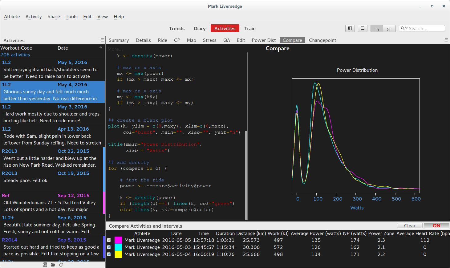
Power Density Plot
Here is a script that plots density distributions for power and is compatible with compare mode:
## R script will run on selection.
##
## GC.activity(compare=TRUE)
## GC.metrics(all=FALSE)
##
## Get the current ride or metrics
##

# get a list of activities, will have one member
# if not in compare mode, or multiple if we are
# in compare mode
d <- GC.activity(compare=TRUE)

## set plot limits
maxy <-0
maxx <-0

for (compare in d) {

   # get the activity being compared
   power <- compare$activity$power

   # density
   k <- density(power)

   # max on x axis
   mx <- max(power)
   if (mx > maxx) maxx <- mx;

   # max on y axis
   my <- max(k$y)
   if (my > maxy) maxy <- my;
}

## create a blank plot
plot(k, ylim = c(0,maxy), xlim=c(0,maxx),
     col="black", main="", xlab="", yaxt="n")

title(main="Power Distribution",
      xlab = "Watts")

## add density
for (compare in d) {

    # just the ride
    power <- compare$activity$power

    k <- density(power)
    if (length(d)==1) lines(k, col="green")
    else lines(k, col=compare$color)
}
As you may have guessed the script in an R chart will be re-run when an activity is selected or compare pane changes (you add or deselect an activity etc).
GC.activity.metrics(compare=FALSE)
Will retrieve a data.frame of the metric and metadata fields for the current activity, provided they are defined in Data Field config with a non blank Screen Tab. This also includes the ride color according to the current config. If compare is true it will return a list.
NOTE there is a metric called Checksum which is a CRC generated for the activity. It is based upon the activity raw data, metadata and start date and time. It will change when the activity data changes and is therefore a useful value to use with the R.cache and memoise R packages for caching previously computed values.
e.g. metrics for the current activity:
> metrics <- GC.activity.metrics()
> str(metrics)
'data.frame': 1 obs. of 301 variables:
$ date : Date, format: "2016-05-05"
$ time : POSIXct, format: "2016-05-05 11:57:18"
$ axPower : num 160
$ aPower_Relative_Intensity : num 0.711
$ aBikeScore : num 53.2
$ Skiba_aVI : num 1.18
$ aPower_Response_Index : num 1.43
$ aNP : num 175
$ aIF : num 0.777
$ aTSS : num 61.7
$ aVI : num 1.29
$ aPower_Efficiency_Factor : num 1.57
$ aTSS_per_hour : num 58.3
$ Aerobic_Decoupling : num 0
$ Activities : num 1
$ To_Exhaustion : num 0
$ Duration : num 3812
$ Time_Moving : num 3673
$ Time_Carrying : num 4
$ Elevation_Gain_Carrying : num 0
$ Distance : num 25.6
$ Distance_Swim : num 25573
$ Climb_Rating : num 1.69
$ Athlete_Weight : num 91.1
$ Athlete_Bodyfat : num 0
$ Athlete_Lean_Weight : num 0
$ Athlete_Bodyfat_Percent : num 0
$ Elevation_Gain : num 208
$ Elevation_Loss : num 202
$ Work : num 497
$ Average_Speed : num 25.1
$ Pace : num 2.39
$ Pace_Swim : num 0.239
$ Average_Power : num 135
$ Average_SmO2 : num 0
$ Average_tHb : num 0
$ Average_aPower : num 136
$ Nonzero_Average_Power : num 159
$ Average_Heart_Rate : num 112
$ Average_Core_Temperature : num 36
$ Heartbeats : num 7.45
$ HrPw_Ratio : num 1.21
$ Workbeat_stress : num 0.037
$ Watts:RPE_Ratio : num 0
$ Power_Percent_of_Max : num 17.3
$ HrNp_Ratio : num 1.55
$ Average_Cadence : num 76
$ Average_Temp : num 21.9
$ Max_Power : num 601
$ Max_SmO2 : num 0
$ Max_tHb : num 0
$ Min_SmO2 : num 0
$ Min_tHb : num 0
$ Max_Heartrate : num 112
$ Min_Heartrate : num 111
$ Max_Core_Temperature : num 37
$ Max_Speed : num 55.7
$ Max_Cadence : num 139
$ Max_Temp : num 25
$ Min_Temp : num 21
$ 95%_Heartrate : num 0
$ VAM : num 196
$ EOA : num 0.692
$ Gradient : num 0.813
$ Average_Power_Variance : num 57.9
$ Max_Power_Variance : num 601
$ Average_Left_Torque_Effectiveness : num 0
$ Average_Right_Torque_Effectiveness : num 0
$ Average_Left_Pedal_Smoothness : num 0
$ Average_Right_Pedal_Smoothness : num 0
$ Average_Left_Pedal_Center_Offset : num 0
$ Average_Right_Pedal_Center_Offset : num 0
$ Average_Left_Power_Phase_Start : num 0
$ Average_Right_Power_Phase_Start : num 0
$ Average_Left_Power_Phase_End : num 0
$ Average_Right_Power_Phase_End : num 0
$ Average_Left_Peak_Power_Phase_Start : num 0
$ Average_Right_Peak_Power_Phase_Start : num 0
$ Average_Left_Peak_Power_Phase_End : num 0
$ Average_Right_Peak_Power_Phase_End : num 0
$ Average_Left_Power_Phase_Length : num 0
$ Average_Right_Power_Phase_Length : num 0
$ Average_Peak_Left_Power_Phase_Length : num 0
$ Average_Right_Peak_Power_Phase_Length: num 0
$ Calories : num 635
$ Aerobic_TISS : num 55.5
$ Anaerobic_TISS : num 1.95
$ CP_setting : num 225
$ xPower : num 159
$ Relative_Intensity : num 0.706
$ BikeScore™ : num 52.5
$ Skiba_VI : num 1.17
$ TISS_Aerobicity : num 96.6
$ Response_Index : num 1.42
$ NP : num 174
$ IF : num 0.772
$ TSS : num 60.8
$ VI : num 1.28
$ Efficiency_Factor : num 1.55
[list output truncated]
>
GC.activity.wbal(compare=FALSE)
Because the W'bal data series is always calculated in 1 second intervals it is not returned with the activity data data.frame -- it would cause problems when data is recorded in 0.5 seconds from a track PM or 1.26s by an old Powertap.
Instead, we return it a simple vector of values, and when using compare mode is in a list in the same way as the other activity data.
e.g. plain, no compare active:
> wbal <- GC.activity.wbal()
> str(wbal)
 num [1:4227] 19000 19000 19000 19000 19000 19000 19000 19000 19000 19000 ...
>
e.g. with compare:
> wc <- GC.activity.wbal(compare=TRUE)
> str(wc)
Dotted pair list of 2
 $ :Dotted pair list of 2
  ..$ activity: num [1:4226] 19000 19000 19000 19000 19000 19000 19000 19000 19000 19000 ...
  ..$ color   : chr "#ff00ff"
 $ :Dotted pair list of 2
  ..$ activity: num [1:4534] 19000 19000 19000 19000 19000 19000 19000 19000 19000 19000 ...
  ..$ color   : chr "#00ffff"
>
GC.activity.xdata(name="", compare=FALSE)
To access the raw XData data series in its own sampling interval, which may differ from other data, without interpolation.
When name="" we return a list of the XData series names present on the corresponding activity and, when name specify an XData group we return a data.frame with one column for each series plus additional columns for time and distance, and when using compare mode is in a list in the same way as the other activity data.
Examples:
> GC.activity.xdata()
[1] "HRV"

> str(GC.activity.xdata("HRV"))
'data.frame': 80988 obs. of 4 variables:
$ time        :POSIXct, format: "2016-02-06 12:04:41" "2016-02-06 12:04:41" ...
$ distance    : num 0 0 0 0 0 0 0 0 0 0 0 0 0 ...
$ HRV_R-R     : num 0.413 0.567 0.563 0.561 0.561 ...
$ HRV_R-R_flag: num -1 -1 -1 -1 -1 -1 -1 -1 ...
GC.activity.meanmax(compare=FALSE)
Mean maximal data is returned in a data.frame, with a column for each data series that has mean max data computed. This is a subset of all the data that can be made available (the cache size is expensive and we don't want to cache data that is never or very, very rarely used).
As with the other activity functions it will return a list of a single data.frame of mean maximal series for the ride.
The series is always computed to 1 second intervals, so the returned data contains peak values from 1s through to the end of the activity
e.g. Mean-max for an activity:
> mm <- GC.activity.meanmax()
> str(mm)
'data.frame':	4228 obs. of  8 variables:
 $ power  : num  557 529 517 504 ...
 $ wpk    : num  6.24 5.93 5.79 5.64 ...
 $ cadence: num  97 97 95 93 ...
 $ speed  : num  53.5 53.2 53 52.6 ...
 $ vam    : num  3600 3600 2400 2700 ...
 $ NP     : num  393 392 391 390 ...
 $ apower : num  559 531 519 506 ...
 $ xpower : num  340 339 338 338 ...
>
GC.activity.intervals(type="", activity=0)
Information for the intervals of the requested type (all by default) in activity (current by default) is returned as a data.frame with columns for name, type, start/stop in seconds, color, selected and all the interval metrics.
New in v3.6 GC.intervalType(type=1) return the localized interval type description to allow language independent filtering of intervals.
The following example uses this information to plot power/cadence in the current activity, but only for the samples corresponding to the intervals selected in the side bar:
laps <- GC.activity.intervals()
act <- GC.activity()

# cond is a boolean vector to mark samples in selected intervals
cond <- (act$seconds<0)
for(i in 1:dim(laps)[1]) {
    if (laps$selected[i]) {
        cond <- cond | ((act$seconds>=laps$start[i]) & (act$seconds<laps$stop[i]))
    }
}

plot(act$power[cond], act$cadence[cond])
title(main="Power/Cadence for Selected Intervals", ylab = "RPM", xlab = "Watts")
Trends
When plotting in the trends view you are looking at data across a date range or season (as selected in the sidebar). These functions return data in that context.
GC.season(all=FALSE, compare=FALSE)
Will return a data.frame of seasons, by default it contains one item for the currently selected season but if all is TRUE it will return all seasons configured, and if compare is TRUE will return all seasons being compared. If compare is TRUE and compare is not active it will return the currently selected season.
NOTE: season colors are always set to gray unless in compare mode, in which case they are the compare mode color, to enable use in a plot legend using legend(legend=season$name, fill=season$color ...).
e.g. list all seasons
> GC.season(all=TRUE)
             name      start        end   color
1    2016 Cycling 2016-04-04 2016-09-01 #7f7f7f
2            2015 2014-07-29 2015-01-11 #7f7f7f
3            2014 2014-07-12 2015-01-23 #7f7f7f
4            2010 2010-01-01 2011-01-01 #7f7f7f
5       Late 2009 2009-04-01 2009-08-01 #7f7f7f
6        Mid 2009 2009-01-01 2009-04-01 #7f7f7f
7      Early 2009 2008-08-01 2009-01-01 #7f7f7f
8            2009 2008-08-01 2009-09-01 #7f7f7f
9            2007 2006-07-01 2007-08-01 #7f7f7f
10      All Dates 1966-05-07 2066-05-07 #7f7f7f
11      This Year 2016-01-01 2016-12-31 #7f7f7f
12     This Month 2016-05-01 2016-05-31 #7f7f7f
13     Last Month 2016-04-01 2016-04-30 #7f7f7f
14      This Week 2016-05-02 2016-05-08 #7f7f7f
15      Last Week 2016-04-25 2016-05-01 #7f7f7f
16    Last 7 days 2016-05-01 2016-05-07 #7f7f7f
17   Last 14 days 2016-04-24 2016-05-07 #7f7f7f
18   Last 21 days 2016-04-17 2016-05-07 #7f7f7f
19   Last 28 days 2016-04-10 2016-05-07 #7f7f7f
20  Last 2 months 2016-03-07 2016-05-07 #7f7f7f
21  Last 3 months 2016-02-07 2016-05-07 #7f7f7f
22  Last 6 months 2015-11-07 2016-05-07 #7f7f7f
23 Last 12 months 2015-05-07 2016-05-07 #7f7f7f
>
GC.season.meanmax(all=FALSE, filter="", compare=FALSE)
As for activity above this will return a data.frame of mean maximals for data series. Since vectors in a data.frame must all have the same length they will be zero padded to the longest series.
If you use all and compare together you will get mean maximals for all activities in a list.
As for GC.activities() you can pass a datafilter to get results for activities that pass a specific rule e.g. 'Data contains "P"' to get results only for rides with power.
e.g. mean maximal for current season:
> mm <- GC.season.meanmax()
> str(mm)
'data.frame':	4228 obs. of  8 variables:
 $ power  : num  557 529 517 504 ...
 $ wpk    : num  6.24 5.93 5.79 5.64 ...
 $ cadence: num  97 97 95 93 ...
 $ speed  : num  53.5 53.2 53 52.6 ...
 $ vam    : num  3600 3600 2400 2700 ...
 $ NP     : num  393 392 391 390 ...
 $ apower : num  559 531 519 506 ...
 $ xpower : num  340 339 338 338 ...
>
Compare Mean Maximal Power
e.g. plotting comparisons of mean maximal power
## plot meanmax
GC.page(width=800,height=600)

## get data
compares <- GC.season.meanmax(compare=TRUE)

plot(compares[1](/GoldenCheetah/GoldenCheetah/wiki/1)$meanmax$power,
     type="n",
     log="xy",
     ylab="Watts",
     xlab="Seconds",
     ylim=c(100,1000), xlim=c(1,10000))

for(compare in compares) {
   points(compare$meanmax$power,
          col=compare$color,
          pch=20)
}
NOTE: when plotting with log scales you cannot set the scales (ylim/xlim) from 0 since log(0) is infinite. Instead in the example above the data is limited to 100 and 1 for Y and X scales respectively.
GC.season.metrics(all=FALSE, filter="", compare=FALSE)
Will fetch the metrics for rides in the currently selected date range, or all dates if all=TRUE. As you would expect the compare parameter will return a list.
As for GC.season.metrics() you can pass a datafilter to get results for activities that pass a specific rule e.g. 'Data contains "P"' to get results only for rides with power.
Of note here are the metadata fields are also returned in the data.frame, provided they are defined in Data Field config with a non blank Screen Tab, a date field as well as a datetime field and the ride color as applied using the GC coloring rules. Color is a text string in "#rrggbb" format.
It is common to use the color column to control coloring on the plots.
e.g. fetching metrics for the current date range:
> metrics <- GC.season.metrics()
> str(metrics)
'data.frame': 245 obs. of 301 variables:
$ date : Date, format: "2008-08-14" "2008-08-16" ...
$ time : POSIXct, format: "2008-08-14 16:45:52" "2008-08-16 12:00:26" ...
$ axPower : num 168 200 211 193 0 ...
$ aPower_Relative_Intensity : num 0.67 0.799 0.845 0.77 0 ...
$ aBikeScore : num 68.1 232.2 123.2 128.1 0 ...
$ Skiba_aVI : num 1.19 1.22 1.23 1.15 0 ...
$ aPower_Response_Index : num Inf 1.39 1.64 1.55 0 ...
$ aNP : num 179 210 221 201 0 ...
$ aIF : num 0.715 0.839 0.884 0.804 0 ...
$ aTSS : num 75.2 254.3 134.6 139.3 0 ...
$ aVI : num 1.27 1.28 1.28 1.2 0 ...
$ aPower_Efficiency_Factor : num Inf 1.46 1.71 1.62 0 ...
$ aTSS_per_hour : num 49.6 63.9 78.1 64.6 0 ...
$ Aerobic_Decoupling : num 0 17.59 15.39 9.27 0 ...
$ Activities : num 1 1 1 1 1 1 1 1 1 1 ...
$ To_Exhaustion : num 0 0 0 0 0 0 0 0 0 0 ...
$ Duration : num 5454 14330 6210 7764 1611 ...
$ Time_Moving : num 5287 12891 6165 7699 520 ...
$ Time_Carrying : num 0 0 0 0 0 0 0 0 118 0 ...
$ Elevation_Gain_Carrying : num 0 0 0 0 0 ...
$ Distance : num 28.48 77.412 33.96 45.284 0.727 ...
$ Distance_Swim : num 28480 77412 33960 45284 727 ...
$ Climb_Rating : num 0 0 0 0 0.235 ...
$ Athlete_Weight : num 89 89 89 89 85 89 89 89 89 89 ...
$ Athlete_Bodyfat : num 0 0 0 0 0 0 0 0 0 0 ...
$ Athlete_Lean_Weight : num 0 0 0 0 0 0 0 0 0 0 ...
$ Athlete_Bodyfat_Percent : num 0 0 0 0 0 0 0 0 0 0 ...
$ Elevation_Gain : num 0 0 0 0 13.1 ...
$ Elevation_Loss : num 0 0 0 0 13.1 ...
$ Work : num 746 2138 1068 1297 0 ...
$ Average_Speed : num 19.65 22.91 20.44 21.86 5.04 ...
$ Pace : num 3.05 2.62 2.93 2.74 11.92 ...
$ Pace_Swim : num 0.305 0.262 0.293 0.274 1.192 ...
$ Average_Power : num 141 164 172 167 0 ...
$ Average_SmO2 : num 0 0 0 0 0 0 0 0 0 0 ...
$ Average_tHb : num 0 0 0 0 0 0 0 0 0 0 ...
$ Average_aPower : num 141 164 172 167 0 ...
$ Nonzero_Average_Power : num 143 176 179 174 0 ...
$ Average_Heart_Rate : num 0 144 129 124 0 ...
$ Average_Core_Temperature : num 0 38 37.9 37.8 0 ...
$ Heartbeats : num 0 31150 13314 16023 0 ...
$ HrPw_Ratio : num 0 1.14 1.33 1.35 0 ...
$ Workbeat_stress : num 0 666 142 208 0 ...
$ Watts:RPE_Ratio : num 0 0 0 0 0 0 0 0 0 0 ...
$ Power_Percent_of_Max : num 15.7 18.3 19.1 18.6 0 ...
$ HrNp_Ratio : num 0 1.46 1.71 1.62 0 ...
$ Average_Cadence : num 64.6 68.9 68.8 76 0 ...
$ Average_Temp : num -255 -255 -255 -255 -255 -255 -255 -255 -255 -255 ...
$ Max_Power : num 692 804 760 647 0 582 731 607 0 692 ...
$ Max_SmO2 : num 0 0 0 0 0 0 0 0 0 0 ...
$ Max_tHb : num 0 0 0 0 0 0 0 0 0 0 ...
$ Min_SmO2 : num 0 0 0 0 0 0 0 0 0 0 ...
$ Min_tHb : num 0 0 0 0 0 0 0 0 0 0 ...
$ Max_Heartrate : num 0 177 170 163 0 170 169 177 171 175 ...
$ Min_Heartrate : num 0 70 59 84 0 82 75 73 65 67 ...
$ Max_Core_Temperature : num 0 38.9 38.4 38.2 0 ...
$ Max_Speed : num 43 59.2 44.1 51 10.1 ...
$ Max_Cadence : num 244 244 244 244 0 244 244 244 0 183 ...
$ Max_Temp : num -255 -255 -255 -255 -255 -255 -255 -255 -255 -255 ...
$ Min_Temp : num -255 -255 -255 -255 -255 -255 -255 -255 -255 -255 ...
$ 95%_Heartrate : num 0 168 158 143 0 161 158 163 168 160 ...
$ VAM : num 0 0 0 0 29.2 ...
$ EOA : num 0 0 0 0 0 0 0 0 0 0 ...
$ Gradient : num 0 0 0 0 1.8 ...
$ Average_Power_Variance : num 89.8 81.4 70.5 69.4 0 ...
$ Max_Power_Variance : num 692 804 747 469 0 535 668 580 0 692 ...
$ Average_Left_Torque_Effectiveness : num 0 0 0 0 0 0 0 0 0 0 ...
$ Average_Right_Torque_Effectiveness : num 0 0 0 0 0 0 0 0 0 0 ...
$ Average_Left_Pedal_Smoothness : num 0 0 0 0 0 0 0 0 0 0 ...
$ Average_Right_Pedal_Smoothness : num 0 0 0 0 0 0 0 0 0 0 ...
$ Average_Left_Pedal_Center_Offset : num 0 0 0 0 0 0 0 0 0 0 ...
$ Average_Right_Pedal_Center_Offset : num 0 0 0 0 0 0 0 0 0 0 ...
$ Average_Left_Power_Phase_Start : num 0 0 0 0 0 0 0 0 0 0 ...
$ Average_Right_Power_Phase_Start : num 0 0 0 0 0 0 0 0 0 0 ...
$ Average_Left_Power_Phase_End : num 0 0 0 0 0 0 0 0 0 0 ...
$ Average_Right_Power_Phase_End : num 0 0 0 0 0 0 0 0 0 0 ...
$ Average_Left_Peak_Power_Phase_Start : num 0 0 0 0 0 0 0 0 0 0 ...
$ Average_Right_Peak_Power_Phase_Start : num 0 0 0 0 0 0 0 0 0 0 ...
$ Average_Left_Peak_Power_Phase_End : num 0 0 0 0 0 0 0 0 0 0 ...
$ Average_Right_Peak_Power_Phase_End : num 0 0 0 0 0 0 0 0 0 0 ...
$ Average_Left_Power_Phase_Length : num 0 0 0 0 0 0 0 0 0 0 ...
$ Average_Right_Power_Phase_Length : num 0 0 0 0 0 0 0 0 0 0 ...
$ Average_Peak_Left_Power_Phase_Length : num 0 0 0 0 0 0 0 0 0 0 ...
$ Average_Right_Peak_Power_Phase_Length: num 0 0 0 0 0 0 0 0 0 0 ...
$ Calories : num 0 3162 1283 1507 0 ...
$ Aerobic_TISS : num 80.2 246.3 125.9 132.2 0 ...
$ Anaerobic_TISS : num 3.3 7.71 4.58 3.39 0 ...
$ CP_setting : num 250 250 250 250 0 250 250 250 0 250 ...
$ xPower : num 168 200 211 193 0 ...
$ Relative_Intensity : num 0.67 0.799 0.845 0.77 0 ...
$ BikeScore™ : num 68.1 232.2 123.2 128.1 0 ...
$ Skiba_VI : num 1.19 1.22 1.23 1.15 0 ...
$ TISS_Aerobicity : num 96 97 96.5 97.5 0 ...
$ Response_Index : num Inf 1.39 1.64 1.55 0 ...
$ NP : num 179 210 221 201 0 ...
$ IF : num 0.715 0.839 0.884 0.804 0 ...
$ TSS : num 75.2 254.3 134.6 139.3 0 ...
$ VI : num 1.27 1.28 1.28 1.2 0 ...
$ Efficiency_Factor : num 0 1.46 1.71 1.62 0 ...
[list output truncated]
>
e.g. looking at the color series, and Workout_Code metadata
> print(metrics$color)
  [1] "#7f7f7f" "#7f7f7f" "#7f7f7f" "#7f7f7f" "#7f7f7f" "#7f7f7f" "#7f7f7f"
  [8] "#7f7f7f" "#7f7f7f" "#7f7f7f" "#7f7f7f" "#7f7f7f" "#7f7f7f" "#7f7f7f"
 [15] "#7f7f7f" "#7f7f7f" "#7f7f7f" "#7f7f7f" "#7f7f7f" "#7f7f7f" "#7f7f7f"
 [22] "#7f7f7f" "#7f7f7f" "#7f7f7f" "#7f7f7f" "#7f7f7f" "#7f7f7f" "#7f7f7f"
 [29] "#7f7f7f" "#7f7f7f" "#7f7f7f" "#7f7f7f" "#7f7f7f" "#7f7f7f" "#7f7f7f"
 [36] "#7f7f7f" "#7f7f7f" "#7f7f7f" "#7f7f7f" "#5555ff" "#7f7f7f" "#5555ff"
 [43] "#5555ff" "#7f7f7f" "#7f7f7f" "#7f7f7f" "#7f7f7f" "#7f7f7f" "#7f7f7f"
 [50] "#7f7f7f" "#5555ff" "#7f7f7f" "#7f7f7f" "#7f7f7f" "#7f7f7f" "#7f7f7f"
 [57] "#7f7f7f" "#5555ff" "#7f7f7f" "#5555ff" "#5555ff" "#7f7f7f" "#7f7f7f"
 [64] "#5555ff" "#7f7f7f" "#5555ff" "#7f7f7f" "#7f7f7f" "#7f7f7f" "#7f7f7f"
 [71] "#7f7f7f" "#7f7f7f" "#7f7f7f" "#7f7f7f" "#7f7f7f" "#7f7f7f" "#7f7f7f"
 [78] "#7f7f7f" "#7f7f7f" "#7f7f7f" "#7f7f7f" "#7f7f7f" "#7f7f7f" "#5555ff"
 [85] "#5555ff" "#7f7f7f" "#5555ff" "#7f7f7f" "#7f7f7f" "#7f7f7f" "#7f7f7f"
 [92] "#7f7f7f" "#5555ff" "#7f7f7f" "#7f7f7f" "#5555ff" "#7f7f7f" "#7f7f7f"
 [99] "#5555ff" "#5555ff" "#7f7f7f" "#7f7f7f" "#7f7f7f" "#7f7f7f" "#5555ff"
[106] "#7f7f7f" "#7f7f7f" "#7f7f7f" "#7f7f7f" "#7f7f7f" "#7f7f7f" "#5555ff"
[113] "#7f7f7f" "#7f7f7f" "#7f7f7f" "#00aa00" "#7f7f7f" "#7f7f7f" "#5555ff"
[120] "#7f7f7f" "#7f7f7f" "#7f7f7f" "#00aa00" "#5555ff" "#7f7f7f" "#7f7f7f"
[127] "#7f7f7f" "#00aa00" "#7f7f7f" "#7f7f7f" "#5555ff" "#00aa00" "#5555ff"
[134] "#7f7f7f" "#7f7f7f" "#00aa00" "#7f7f7f" "#7f7f7f" "#00aa00" "#7f7f7f"
[141] "#7f7f7f" "#00aa00" "#7f7f7f" "#7f7f7f" "#7f7f7f" "#7f7f7f" "#7f7f7f"
[148] "#7f7f7f" "#7f7f7f" "#7f7f7f" "#5555ff" "#7f7f7f" "#7f7f7f" "#00aa00"
[155] "#7f7f7f" "#7f7f7f" "#7f7f7f" "#7f7f7f" "#7f7f7f" "#00aa00" "#7f7f7f"
[162] "#00aa00" "#7f7f7f" "#7f7f7f" "#00aa00" "#00aa00" "#7f7f7f" "#7f7f7f"
[169] "#7f7f7f" "#5555ff" "#7f7f7f" "#00aa00" "#7f7f7f" "#7f7f7f" "#7f7f7f"
[176] "#7f7f7f" "#5555ff" "#7f7f7f" "#7f7f7f" "#7f7f7f" "#7f7f7f" "#00aa00"
[183] "#7f7f7f" "#7f7f7f" "#7f7f7f" "#7f7f7f" "#00aa00" "#5555ff" "#5555ff"
[190] "#7f7f7f" "#00aa00" "#7f7f7f" "#7f7f7f" "#7f7f7f" "#5555ff" "#7f7f7f"
[197] "#7f7f7f" "#00aa00" "#7f7f7f" "#00aa00" "#7f7f7f" "#5555ff" "#7f7f7f"
[204] "#5555ff" "#7f7f7f" "#00aa00" "#7f7f7f" "#7f7f7f" "#7f7f7f" "#7f7f7f"
[211] "#7f7f7f" "#7f7f7f" "#7f7f7f" "#5555ff" "#5555ff" "#7f7f7f" "#00aa00"
[218] "#7f7f7f" "#7f7f7f" "#7f7f7f" "#5555ff" "#7f7f7f" "#7f7f7f" "#5555ff"
[225] "#00aa00" "#7f7f7f" "#5555ff" "#5555ff" "#ff00ff" "#5555ff" "#5555ff"
[232] "#7f7f7f" "#00aa00" "#7f7f7f" "#7f7f7f" "#7f7f7f" "#7f7f7f" "#7f7f7f"
[239] "#7f7f7f" "#7f7f7f" "#7f7f7f" "#7f7f7f" "#7f7f7f" "#7f7f7f" "#00aa00"
> print(metrics$Workout_Code)
  [1] ""       ""       ""       ""       ""       ""       ""       ""
  [9] ""       ""       ""       ""       ""       ""       ""       ""
 [17] ""       ""       ""       ""       ""       ""       ""       ""
 [25] ""       ""       ""       ""       ""       ""       ""       ""
 [33] "1L3+"   "3L3+"   "1L3"    "2L3"    "2L3"    "1L3"    "3L2+"   "2SST"
 [41] "2L3+"   "2SST+"  "2SST"   "2L3"    "2L2"    "1L3"    "1L3"    "1L3"
 [49] "1L3"    "1L3+"   "1SST"   "1L3"    "1L3"    "1L3"    "2L3+"   "2L3"
 [57] "2L3+"   "FTP"    "1AR"    "1SST"   "1SST"   "2L3+"   "1L3"    "1SST"
 [65] "2L3"    "2SST"   "2L3"    "1AR"    "2L2+"   "1AR"    "1L3+"   "1L2"
 [73] "2L3"    "2L2"    "2L1"    "3L2+"   "2L3"    "WARM"   "1L3"    "2L3"
 [81] "2L3"    "2L2+"   "WARM"   "2x20L4" "1L4"    "WARM"   "220L4"  "2L3+"
 [89] "2L3"    "WARM"   "1L3"    "90P234" "FTP"    "WARM"   "2L3"    "90SST"
 [97] "WARM"   "2P234"  "1SST"   "2SST"   "1L3"    "90L3"   "90L3"   "1L3"
[105] "FTP"    "2L2"    "90L3+"  "50G3"   "1G7"    ""       "1L2"    "FTP"
[113] "2L3"    "2L3"    "2L3"    "2HILLS" "90AR"   "2L3+"   "2L4"    "2L3"
[121] "1AR"    "1AR"    "4HILLS" "FTP"    "2L3"    "2L3"    "1AR"    "3HILLS"
[129] "1L3"    "2L3"    "1SST"   "1HILLS" "FTP"    "2L3"    "90L3"   "2HILLS"
[137] "90L2"   "fun"    "2HILLS" ""       "1L2"    "1HILLS" "1L3"    "2L3"
[145] "2L3"    "2AR"    "1AR"    "90I3"   "WARM"   "1L3"    "2SST"   "2L3"
[153] "2L3"    "2HILLS" "WARM"   "1L3"    "1L3"    "1L3"    "2L3"    "5HILLS"
[161] "1AR"    "3HILLS" "1L3"    ""       "1HILLS" "1HILLS" "1L3"    "2L3"
[169] "1AR"    "FTP"    "2L3"    "1HILLS" "2L3"    "2L3"    "2L2"    "1L3"
[177] "1SST"   "1AR"    "2L3"    "2L3"    "2L2"    "3HILLS" "2L2"    "2L2"
[185] "1L2+"   "1L3"    "6HILLS" "1SST"   "FTP"    "1AR"    "2HILLS" "1L3"
[193] "1AR"    "2L3"    "1SST"   "2L2"    "2AR"    "2HILLS" "2AR"    "1HILLS"
[201] ""       "1SST"   "1L3"    "1SST"   "2AR"    "3HILLS" "1AR"    "1AR"
[209] ""       "2L3"    "2L3"    "2L3"    "1AR"    "1SST"   "1SST"   "1L3"
[217] "2HILLS" "1L3"    ""       "1L3"    "1SST"   "2L3"    "3L2"    "1SST"
[225] "1HILLS" "2L2"    "1SST"   "1SST"   "RACE"   "1SST"   "1SST"   "1L3"
[233] "2HILLS" "2L3"    ""       "1L2"    "1L2"    ""       "1L2"    ""
[241] ""       ""       ""       "1L2"    "2HILLS"
>
GC.season.peaks(all=FALSE, filter="", compare=FALSE, series, duration)
To get the peaks for all activities in a season, the series should be a name for which mean maximal data is available ("power", "heart.rate", "speed" et al) and the duration should be the duration is seconds.
It will return a data.frame with vectors for each series+duration combination as well as a datetime vector for the datetime the peak was recorded. Bear in mind there will be one peak for every activity, rather than per day.
As for GC.season.metrics() you can pass a datafilter to get results for activities that pass a specific rule e.g. 'Data contains "P"' to get results only for rides with power.
As with most of the methods compare=TRUE will return a list for each date range being compared or the current date range if compare is not active.
e.g. get some heartrate and power peaks:
> peaks <- GC.season.peaks(series=c("power", "heart.rate"), duration=c(1,10,100,1000))
> str(peaks)
'data.frame':	74 obs. of  9 variables:
 $ time                : POSIXct, format: "2008-08-14 16:45:52" "2008-08-16 12:00:26" ...
 $ peak_power_1        : num  692 804 760 647 0 582 731 607 0 692 ...
 $ peak_power_10       : num  509 668 606 595 0 ...
 $ peak_power_100      : num  245 322 296 267 0 ...
 $ peak_power_1000     : num  158 223 229 194 0 ...
 $ peak_heart.rate_1   : num  0 177 170 163 0 170 169 177 171 175 ...
 $ peak_heart.rate_10  : num  0 176 169 163 0 ...
 $ peak_heart.rate_100 : num  0 174 165 148 0 ...
 $ peak_heart.rate_1000: num  0 154 149 131 0 ...
>
GC.season.pmc(all=FALSE, metric="TSS")
To fetch PMC metrics for the currently selected date range, or all dates if all=TRUE, this method returns a data.frame containing columns for all the PMC metrics series and additionally a date column.
You can specify a metric to use (TSS is used by default).
e.g. PMC data using Work (Joules) as the input:
> pmc<-GC.season.pmc(metric="Work")
> str(pmc)
'data.frame':	397 obs. of  6 variables:
 $ date  : Date, format: "2008-08-01" "2008-08-02" ...
 $ stress: num  0 0 0 0 0 0 0 0 0 0 ...
 $ lts   : num  28.9 28.2 27.5 26.9 26.3 ...
 $ sts   : num  14.67 12.72 11.03 9.56 8.29 ...
 $ sb    : num  12.6 14.2 15.5 16.5 17.3 ...
 $ rr    : num  -5.24 -5.11 -4.99 -4.88 -4.76 ...
>
PMC and Metric Plotting together
Putting metrics and pmc together and using some R base graphics, here is an example plot that plots each activity in term of the intensity (IF) and training freshness (TSB) with each dot in the scatter plot representing overall stress of the ride (TSS).
Note how the PMC and Metric data is merged, this is using stock R functionality and relies on the common 'date' field in the metrics and pmc data.frames.
Also note how the shorthand functions GC.metrics() and GC.pmc() are being used instead of GC.season.metrics() and GC.season.pmc()
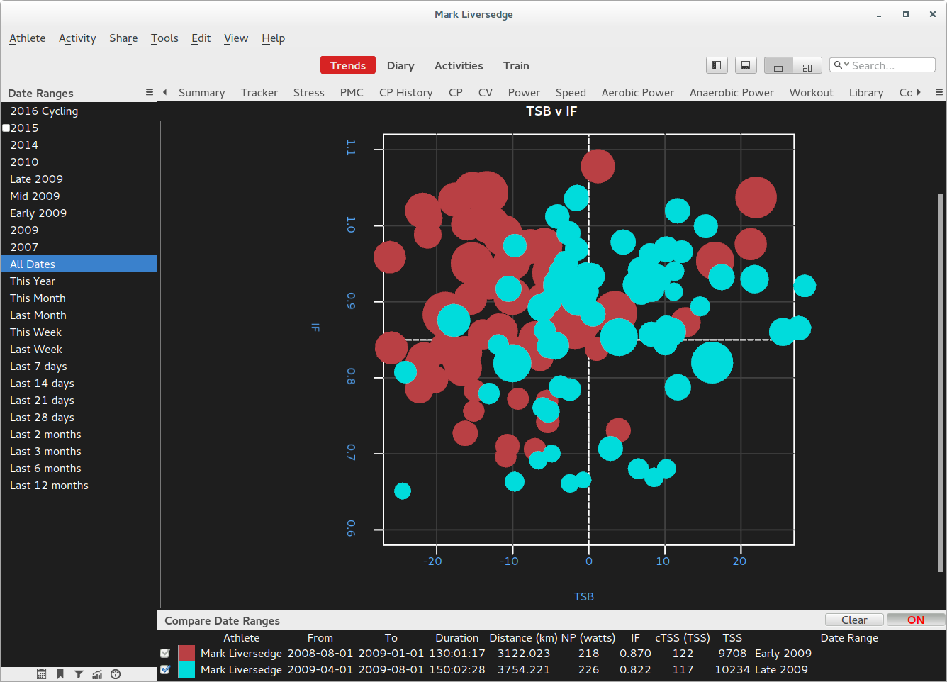
Its an interesting way of reviewing PMC data, especially when you compare the makeup of one training block with another.
##
## TSB v IF with TSS
##
## How fresh were we and how hard did we go
## and how much stress did we elicit.
## A more meaningful way of reviewing the
## PMC data in terms of managing load/intensity

GC.page(width=800, height=600)

## get data
compares <- GC.season.metrics(compare=TRUE)

## all pmc data
pmc <- GC.season.pmc(all=TRUE, metric="cTSS")

# bigger margins please
par(mar=c(6,6,6,6))

plot(x=c(-30), y=c(0),
     ylim=c(0.6,1.1), xlim=c(-60,+60),
     xlab="", main="", ylab="")

## grid lines
grid(col="#404040", lty="solid", lwd=1)

## title
title(main="",
      xlab="TSB",
      ylab="IF")

## abline
abline(h=0.85, slope=0, lty="dashed", col="white")
abline(v=0, slope=1, lty="dashed", col="white")

for (compare in compares) {

    # combine pmc and metric data
    z <- merge(compare$metrics, pmc, by="date")

    # area of circle should be proportional
    radius <- sqrt( z$cTSS/ 3.1415927 )

    # plot using ride colors if not comparing
    # or only one date range selected
    if (length(compares) == 1) {

        # make transparent for overlapping
        colors <- adjustcolor(z$color, 0.6)

        symbols(z$sb, z$IF,
                circles=radius,
                inches=0.4,
                add=TRUE,
                bg=colors,fg=colors,
                xlab="", ylab="")
    } else {

        # make transparent for overlapping
        color <- adjustcolor(compare$color, 0.6)

        symbols(z$sb, z$IF,
                circles=radius,
                inches=0.4,
                add=TRUE,
                bg=color,
                fg=color,
                xlab="", ylab="")


    }

    # labels for each bubble
    ##text(z$"4", z$IF, z$Workout_Code, col="gray", cex=0.5)
}

## name the quadrants
text(-30,0.6, "Maintain", col="darkgray", cex=1)
text(30,1.09, "Race", col="darkgray", cex=1)
text(-30,1.09, "Overload", col="darkgray", cex=1)
text(30,0.6, "Junk", col="darkgray", cex=1)
GC.season.intervals(type="", compare=FALSE)
Note: this call was introduced in v3.5 of GoldenCheetah
To fetch details of all intervals across all activities for a season. The response is pretty much the same as you would see for GC.season.metrics() with the exception that each row represents an interval and not an activity.
In addition to the metrics each row also contains the interval type and the interval name. The interval type will be one of:
- ALL - an interval that represents an entire activity
- DEVICE - an interval specific to the device e.g. calibration points
- USER - a user defined interval
- PEAK PACE - a section of an activity that was peak pace for a specific duration
- PEAK POWER - a section of an activity that was peak power for a specific duration
- SEGMENTS - a segment found that represents a specific route using GPS
- CLIMBING - an ascent that was automatically marked
- EFFORTS - an automatically detected maximal effort
New in v3.6 GC.intervalType(type=1) return the localized interval type description to allow language independent filtering of intervals.
GC.season.measures(all=FALSE, group="Body")
To fetch daily measures for the currently selected date range, or all dates if all=TRUE, this method returns a data.frame containing columns for all the measures group fields and additionally a date column.
You can specify the measure group to fetch, for v3.5 "Body" and "Hrv" are available.
e.g. Hrv measures for the selected date range:
> hrv<-GC.season.measures(group="Hrv")
> str(hrv)
'data.frame'     : 84 obs. of  9 variables:
 $ date          : Date, format: "2017-09-11" "2017-09-12" ...
 $ HR            : num  44.4 44.2 ...
 $ AVNN          : num  1342 1417 ...
 $ SDNN          : num  64.2 61.9 ...
 $ RMSSD         : num  36.4 56.2 ...
 $ PNN50         : num  16.3 22.5 ...
 $ LF            : num  0.0461 0.0493 ...
 $ HF            : num  0.0207 0.0223 ...
 $ RecoveryPoints: num  7.46 8.09 ...
Charts
From version 3.6 onwards you can now plot into an interactive chart withing goldencheetah. This allows the user to interact with data points and axes as well as annotate. The overall user experience reflects the rest of goldencheetah and provides a more natural way for users to work. We strongly recommend that you develop new charts using this and avoid plotting to the R graphics device.
In general terms, the API for working with charts should be called in sequence;
GC.setChart(..)to define the kind of chart and basic settings firstGC.addCurve(..)to add data to the chart with implicit axis namesGC.annotate(..)to add other kinds of data to the chartGC.setAxis(..)at the end to configure the axes used by the curves
NOTE: Most crucially, you must call setAxis(..) AFTER adding all the curves.
GC.setChart(title, type, animate, legpos, stack, orientation)
title defaults to 1 and it will be displayed at the top of the chart otherwise.
type defaults to 1 and it can be one of:
- GC.CHART.LINE=1
- GC.CHART.SCATTER=2
- GC.CHART.BAR=3
- GC.CHART.PIE=4
- GC.CHART.STACK=5
- GC.CHART.PERCENT=6
animate setting defaults to false and it has been reported to provoke crashes is some setups, if you are experiencing them, please disable animation.
legpos defaults to 2 and it can be one of:
- GC.ALIGN.BOTTOM=0
- GC.ALIGN.LEFT=1
- GC.ALIGN.TOP=2
- GC.ALIGN.RIGHT=3
- GC.ALIGN.NONE=4
so legend which can be placed at the top, bottom, left or right of the chart. It can also be set to 'none' which hides the legend from view.
stack defaults to False
orientation defaults to 1 and it can be one of:
- GC.HORIZONTAL=1
- GC.VERTICAL=2
The layout direction controls whether separate charts are laid out left to right horizontally or top to bottom vertically. Multiple charts are created when different x-axes are used or series are put into 'groups'.
GC.addCurve(name, x, y, f, xaxis, yaxis, labels, colors, line, symbol, size, color, opacity, opengl, legend, datalabels, fill)
name is mandatory
x and y are the lists of x and y values, it should have the same dimension
f is a list of filenames for click-thru on a trends chart, it should have the same dimension as x and y
xaxis is the x-axis name, it defaults to "x"
yaxis is the y-axis name, it defaults to "y"
labels is an optional list of labels
colors is an optional list of colors
line style defaults to 1, and it can take the following values:
- GC.LINE.NONE=0
- GC.LINE.SOLID=1
- GC.LINE.DASH=2
- GC.LINE.DOT=3
- GC.LINE.DASHDOT=4
symbol type defaults to 1, and it can take the following values:
- GC.SYMBOL.NONE=0
- GC.SYMBOL.CIRCLE=1
- GC.SYMBOL.RECTANGLE=2
size is the size/width
color defaults to "cyan"
opacity defaults to 0
opengl defaults to True, it means opengl will be used for rendering. This is very fast and highly recommended for plotting sample by sample data. One of the drawbacks of this is the opengl functions used tend to ignore most of the aesthetic options like transparency and datalabels.
legend defaults to True, and it means this series will be displayed on legend
datalabels defaults to False, and it means data labels will not be displayed
fill defaults to False, and it means the curve will not be filled
GC.setAxis(name, visible, min, max, type, labelcolor, color, log)
name is mandatory and it should match one of the previously added curves axes names.
visible defaults to True
align can be one of:
- GC.ALIGN.BOTTOM=0
- GC.ALIGN.LEFT=1
- GC.ALIGN.TOP=2
- GC.ALIGN.RIGHT=3
- GC.ALIGN.NONE=4
min and max default to -1 meaning automatic
type can take one of the following values:
- GC.AXIS.CONTINUOUS=0 (default)
- GC.AXIS.DATE=1 for x-axes on Trends charts
- GC.AXIS.TIME=2 for x-aces on Activity charts
- GC.AXIS.CATEGORY=3 for bar and pie charts
labelcolor and color are optional
log defaults to False, when True a log scale is used, valid only for GC.AXIS_CONTINUOUS type
categories is an optional list of labels for GC.AXIS_CATEGORY type
GC.annotate(type, series, label, value)
For future versions, unimplemented in v3.6
Example: Omni-domain power duration model
This example was written by Mike Puckowicz and Dave Clarke to support their paper, it has been adapted to use the Qt charting API.
## omnidomain power model

## Get MMP data
MMP <- GC.season.meanmax(all=FALSE, compare=FALSE)$power

# wrangle
len <- length(MMP)
df <- data.frame(matrix(ncol = 2, nrow = (log(len/7.5))/.05))
colnames(df)<- c("time", "power")
df$power[1:20] <- MMP[2:21]
df$time[1:20] <- seq(from = 1, to = 20, by = 1)

n <- 22
while(n <= length(df$power) ){
  i <- 7.5*exp(n*.05)
  df$power[n]<-MMP[round(i)]
  df$time[n]<-round(i)
  n <- n + 1
}

## rename df columns x and y for convenience in the model
colnames(df)<- c("x", "y")

## set start values for parameters
startPmax <- 1000
startW <- 10000
startCP <- 200
startA <- 30

## Crop
MaxTime <- 7200
cut <- round(log(MaxTime/7.5)/.05)
df<- df[1:cut,]

## model fit
form <- as.formula( y~W1/x*(1-exp(-x/(W1/(Pmax-CP)))) + CP - A*(log(x/1800))*(x>1800) )
mod <- nls(form, data=df, start=list(W1=startW, Pmax=startPmax, CP=startCP, A=startA))
mod

## Plot onto Qt Chart
GC.setChart(title="Omni-domain Power Duration Model",
            type=GC.CHART.LINE)

GC.addCurve(name="Bests", xseries=df$x, yseries=df$y,
            xname="Seconds", yname="Watts",
            symbol=0, line=GC.LINE.DOT, size=2, color="gold",
            opengl=FALSE)

GC.addCurve(name="Model", xseries=df$x,
            yseries=predict(mod, newdata=df),
            xname="Seconds", yname="Watts",
            symbol=0, line=GC.LINE.SOLID, size=2, color="red")

GC.annotate(type="label", series="Model",
            c("CP", round(coef(mod)[3])))
GC.annotate(type="label", series="Model",
            c("W1", round(coef(mod)[1])))
GC.annotate(type="label", series="Model",
           c("Pmax", round(coef(mod)[2])))
GC.annotate(type="label", series="Model",
           c("A", round(coef(mod)[4])))


GC.setAxis(name="Seconds", min=1,max=10000, log=TRUE)
GC.setAxis(name="Watts", min=0, max=1000)
BACK: Special Topics: Overview
BACK: Table of contents