UG_Special Topics_Working with Python - GoldenCheetah/GoldenCheetah GitHub Wiki
Below you will find details of each of the GC functions available to use within the Python chart.
- GC.version() to get a version string
- GC.build() to get a build number
- GC.webpage(filename) to set the webpage
- GC.athlete() to get the athlete details
- GC.athleteZones(date=0, sport="") to get zone config
- GC.activities(filter="") to get a list of activities (as dates)
- GC.activity(join="repeat", activity=None, compareindex=-1) to get the activity data
- GC.series(type, activity=None, compareindex=-1) to get an individual series data
- GC.activityWbal(activity=None, compareindex=-1) to get wbal series data
- GC.xdataNames(name="", activity=None, compareindex=-1) to get activity xdata series names
- GC.xdataSeries(name, series, activity=None, compareindex=-1) to get activity xdata series in its own sampling interval
- GC.xdata(name, series, join="repeat", activity=None, compareindex=-1) to get interpolated activity xdata series
- GC.activityMetrics(compare=False) to get the activity metrics and metadata
- GC.activityMeanmax(compare=False) to get mean maximals for all activity data
- GC.activityIntervals(type="", activity=None) to get information about activity intervals
- GC.season(all=False, compare=False) to get season details
- GC.seasonMetrics(all=False, filter="", compare=False) to get season metrics
- GC.seasonMeanmax(all=False, filter="", compare=False) to get best mean maximals for a season
- GC.seasonPeaks(all=False, filter="", compare=False, series, duration) to get activity peaks for a given series and duration
- GC.seasonPmc(all=False, metric="TSS") to get PMC data for any given metric
- GC.seasonIntervals(type="", compare=False) to get metrics for all intervals
- GC.seasonMeasures(all=False, group="Body") to get Daily measures (Body and Hrv available for v3.5)
- GC.setChart(...) to setup chart basics
- GC.addCurve(...) to add a curve to the chart
- GC.setAxis(...) to control axis settings
- GC.annotate(...) to add an annotation to the chart
- An interactive chart example with Code
New in v3.6: GoldenCheetah v3.6 builds include Python 3.7, with required and recommended modules pre-installed, to allow easier access to curated Python charts on CloudDB for non-technical users. To use it check Enable Python, leave Python Home empty in options and restart GC, save and restart GC. For advanced users, willing to install additional packages, a separate Python installation is recommended, as documented below.
Python embedding is the most powerful and flexible way to extend GoldenCheetah, but that flexibility comes with a price; to use it you need to know or be willing to learn about Python. Even to use Python charts developed by others, the minimum is to be able to install Python, configure for embedding in GoldenCheetah and manage Python packages using the standard Python package manager (PIP) at the command line in your OS, some script debugging abilities may be necessary. There are lots of freely available resources to educate yourself on these topics, please use them.
Simpler alternatives are available, s.t. in decreasing order of complexity and flexibility: R Charts, User Charts, Metrics Trends Charts and User Data/Custom Metrics with formulas, and configurable standard charts.
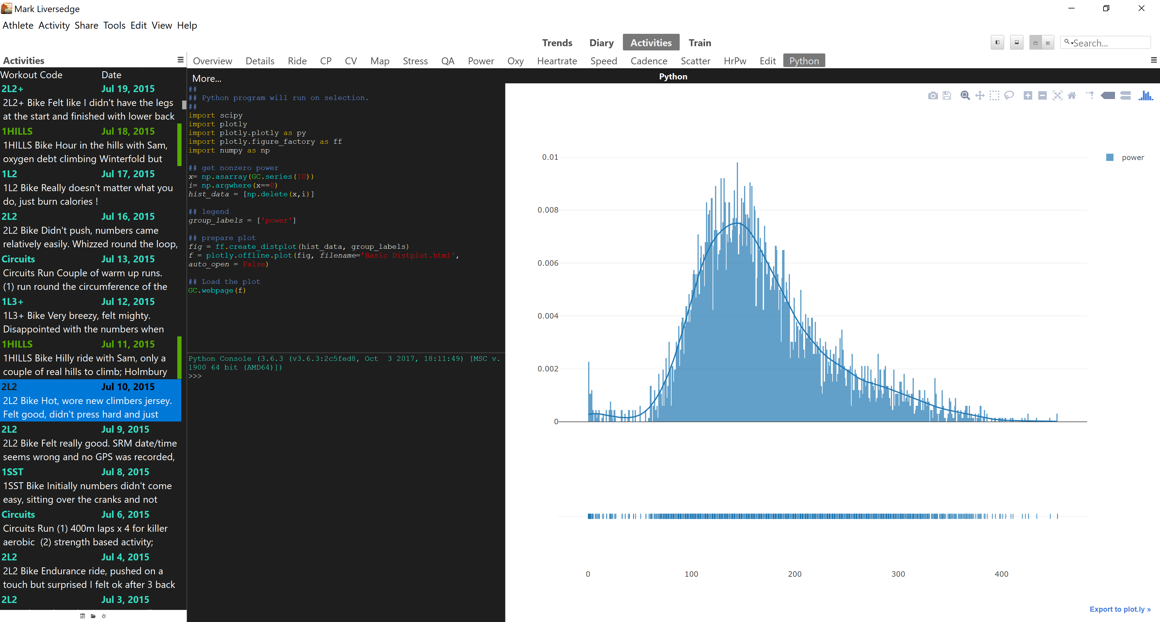
Python chart is introduced with v3.5 of GoldenCheetah and it can be used in activity view and trend view.
We build binaries using Python v3.x and they are only compatible with this release, we do not support embedded use of Python 2.7. Since Python is embedded the runtime must match the versions supported by each release of GoldenCheetah, currently at least major and minor Python version (s.t. 3.6) must match the one reported in Help > About > Versions, if you are experiencing problems we recommend to install exactly the same version informed there.
If Python is not installed in (OS dependent) standard locations or present in PATH, the location needs to be configured in Preferences before to enable Python integration. Python venv/virtualenv are not supported.
The path you need to configure Python in GoldenCheetah can be obtained running the Python interpreter and executing the following commands:
import sys
sys.exec_prefix
After you configure Python in GoldenCheetah, restart GoldenCheetah and check Python is recognized in Help > About > Versions.
Note for v3.6 on Windows: to use your own Python installation with GoldenCheetah v3.6, instead of the included one, it is necessary to remove/rename python37._pth file parallel to GoldenCheetah.exe, this file is part of Python embeddable distribution and blocks access to other Python installations when present.
We recommend using `pip' to install and manage python modules and expect the pip module to have been installed. We highly recommend installing this following modules since they are assumed to be available when developing charts:
GoldenCheetah Integration (required)
- sip (must be version 4.19.x, e.g.
pip install sip==4.19.8)
Data processing
- numpy
- pandas (recommended version 1.2.3, e.g.
pip install pandas==1.2.3)
Data analysis, modelling and learning
- scipy
- scikit-learn
- tensorflow
- lmfit
Visualisation
- colour
- plotly
In trend view the chart is refreshed when a date range or season is selected, or if the compare pane is updated. Whilst in the activity view the chart is refreshed when an activity is selected or, again, if the compare pane for intervals is updated.
When the chart is refreshed the user supplied Python script is executed, and it can collect data using calls via a python API provided by GoldenCheetah (GC), prepare a plot and then render it as a web page.
Since there is no standard graphics system available in python we have chosen to provide two options, which are configuralble in the chart settings; firstly, you can render via the native charting system or secondly via a web browser. So the python script should use APIs listed below for working with the local graphics system or generate some form of html output that can be loaded by the browser. Since there are a fair number of python modules for plotting and visualisation via a browser, we have chosen to standardise on plotly since it is so popular and capable.
Plotly is built using d3.js and stack.gl. The web library plotly.js is a high-level, declarative charting library. plotly.js ships with 20 chart types, including 3D charts, statistical graphs, and SVG maps all of which can be rendered in the python chart's webview.
There are a good number of alternatives to plotly you might consider using such as bokeh, pygal and ggplot. We recommend using plotly wherever possible to avoid additional dependencies if you choose to share your chart with other users via the cloudDB.
A simple example to plot a cadence and power scatter plot:
##
## Python program will run on selection.
##
import numpy as np
import plotly
from plotly.graph_objs import Scatter, Layout
import tempfile
import pathlib


## Retrieve power and cadence
xx = np.asarray(GC.series(GC.SERIES_WATTS))
yy = np.asarray(GC.series(GC.SERIES_CAD))

# Define temporary file
temp_file = tempfile.NamedTemporaryFile(mode="w+t", prefix="GC_", suffix=".html", delete=False)

## Prepare Plot
plotly.offline.plot({
    "data": [Scatter(x=xx, y=yy, mode = 'markers')],
    "layout": Layout(title="Power / Cadence")
}, auto_open = False, filename=temp_file.name)

## Load Plot
GC.webpage(pathlib.Path(temp_file.name).as_uri())
This basically calls a GC function to fetch the data for the current ride and then puts the data into numpy arrays so that plotly can prepare a plot, before rendering it on the chart webpage.
For details on rendering via the local graphics system see the section at the bottom of this page entitled 'Charts'
Local Data, $$ and avoiding data refresh
All data objects are shared across charts. If you create a vector 'x' in one chart it will be available in all the others. Usually, this is not a problem since you fetch the data manipulate it and plot it. But in some cases, where perhaps you prepare data from across the ride data you may want to avoid refreshing it to save time.
If you prefix variable names with $$ then they will get a prefix added to them internally that makes them local to the chart. e.g. $$d internally becomes 'gc0d' on the first chart, 'gc1d' on the second and so on.
We recommend you always prefix variables with $$ to ensure there is not conflict across charts.
Python globals() function is useful to check if a variable was previously set, for example in the following fragment:
if not $$d in globals():
    $$d = some_slow_computation()
print($$d)
the function some_slow_computation() runs only on the fist chart refresh.
Compare Mode
Where applicable the data access routines will offer a 'compare' parameter to access data; if False it just returns the currently selected ride, if True it will return a list. If compare mode is not active then the list will contain only one set of data for the currently selected ride. If compare is active it returns a list of all things being compared. See GC.activity(compare=True) below for an example.
Search/Filtering
If a search or data filter is active then this will be applied to the results returned by the API methods described below. Even when all=True is set to override season date ranges the filter will be applied. Ultimately, if the user doesn't want a filter to be applied they should clear it. We work this way to ensure consistency across all charts.
Stopping long running scripts
Hitting the ESC key will terminate any long running scripts. This can be useful when processing large volumes of data or an errant script runs into an infinite loop. In general, we would recommend letting long running processes complete, but ESC will terminate them safely.
Copy from the console
Normal selection is disabled in the console output for technical reasons, but you can use Ctrl+A to select and Ctrl-Insert to copy the console contents.
Line breaks in string constants
If you need to use a newline character in a string constant, please use chr(10) since ‘\n’ will break the script after restart.
Keywords to avoid
There are no limitations on the python modules or language features that you can use. But you should avoid using commands that require an interactive shell (since there isn't one), so help, copyright etc will hang the interpreter and GoldenCheetah. You should avoid using quit() (or equivalents) since they will terminate GoldenCheetah immediately and may lead to data loss.
Avoiding blocking
Any blocking action, s.t. waiting for user input or starting a synchronous server, will block GoldenCheetah user interface and it should be avoided, the chart script should terminate as soon as possible. Python treading module can be used for that purpose if necessary.
IPython and Jupyter
In the current release we do not support use of the IPython package. Importing IPython and running embed() in a Python chart console (or script) will hang GoldenCheetah. We will be supporting Jupyter Notebooks in releases after version 3.6 of GoldenCheetah and are looking at this actively.
Using IDE for Python chart development
IDEs are not supported inside GC, but there is an independent development enabling creation and debugging of GC Python chart using Python IDEs, see https://github.com/rb83421/GoldenCheetah_Python_Chart_Wrapper
All methods to access and work with GC objects and data within a Python chart are prefixed with "GC." this is to ensure there is no namespace clash with other packages you may have installed. There are a number of methods available as listed below.
GC.build will return the build number which increments with each release (including pre-release development builds), you can use this if you need to make a script dependant on the build. Additionally, GC.version will return a string describing the release,which could be put in files or on screen etc.
The web browser loads and displays the file filename, it is recommended that this is an html file to ensure cross-platform compatibility but that is not mandated.
GC.athlete() will return a dict of athlete details including name, home directory, gender, height, weight and date of birth.
e.g.
>>> print(GC.athlete())
{'height': 1.709, 'weight': 67.0, 'gender': 'male', 'dob': datetime.date(1962, 11, 11), 'name': 'Ale', 'home': '/home/ale/.goldencheetah/Ale'}
Will return a dict of the zone configuration by sport in chronological order. The pace, heartrate and power settings are folded together by sport.
You can specify a date you want to get configuration for, or limit to zone config for a specific sport.
Introduced in v3.6: hrzoneslow and pacezoneslow, similar to zoneslow but for HR and Pace, respectively.
e.g.
>>> print(GC.athleteZones().keys())
dict_keys(['pmax', 'cp', 'date', 'ftp', 'zonescolor', 'zoneslow', 'cv', 'hrmax', 'rhr', 'sport', 'wprime', 'lthr'])
where zonescolor and zoneslow are lists with an element for each Zone.
If you prefer to use Pandas the dict can be easily converted to a Data Frame:
e.g.
>>> import pandas as pd
>>> df = pd.DataFrame(GC.athleteZones())
>>> print(df)
       cp    cv        date    ftp  hrmax   lthr    pmax   rhr sport   wprime  \
0     0.0   3.0  2000-01-01    0.0    0.0    0.0     0.0   0.0  swim      0.0
1     0.0  15.0  2000-01-01    0.0  176.0  158.0     0.0  50.0   run      0.0
2   240.0   0.0  2000-01-01  240.0  170.0  150.0  1000.0  50.0  bike  20000.0
3   170.0   0.0  2012-10-01  170.0  170.0  150.0  1000.0  50.0  bike  20000.0
4   180.0   0.0  2012-10-29  180.0  170.0  150.0  1000.0  50.0  bike  20000.0
5   190.0   0.0  2012-11-26  190.0  170.0  150.0  1000.0  50.0  bike  20000.0
6   200.0   0.0  2012-12-24  200.0  170.0  150.0  1000.0  50.0  bike  20000.0
7   210.0   0.0  2013-01-21  210.0  170.0  150.0  1000.0  50.0  bike  20000.0
8   220.0   0.0  2013-02-18  220.0  170.0  150.0  1000.0  50.0  bike  20000.0
9   230.0   0.0  2013-03-18  230.0  170.0  150.0  1000.0  50.0  bike  20000.0
10  240.0   0.0  2013-04-15  240.0  170.0  150.0  1000.0  50.0  bike  20000.0
11  230.0   0.0  2013-07-15  230.0  170.0  150.0  1000.0  50.0  bike  20000.0
12  220.0   0.0  2013-08-12  220.0  170.0  150.0  1000.0  50.0  bike  29000.0
13    0.0  13.0  2013-12-30    0.0  176.0  158.0     0.0  50.0   run      0.0
14    0.0  13.0  2014-01-27    0.0  176.0  158.0     0.0  50.0   run      0.0
15  230.0   0.0  2014-02-03  230.0  170.0  150.0  1000.0  50.0  bike  20000.0
16    0.0  14.0  2014-03-24    0.0  176.0  158.0     0.0  50.0   run      0.0
17    0.0  13.0  2014-04-24    0.0  176.0  158.0     0.0  50.0   run      0.0
18    0.0  14.0  2014-05-19    0.0  176.0  158.0     0.0  50.0   run      0.0
19    0.0  14.0  2014-06-16    0.0  176.0  158.0     0.0  50.0   run      0.0
20    0.0  15.0  2014-07-14    0.0  176.0  158.0     0.0  50.0   run      0.0
21  240.0   0.0  2014-07-14  240.0  170.0  150.0  1000.0  50.0  bike  20000.0
22    0.0  15.0  2014-08-11    0.0  176.0  158.0     0.0  50.0   run      0.0
23  250.0   0.0  2014-09-29  250.0  170.0  150.0  1000.0  50.0  bike  20000.0
24  240.0   0.0  2014-11-17  240.0  170.0  150.0  1000.0  50.0  bike  20000.0
25  230.0   0.0  2014-12-28  230.0  170.0  150.0  1000.0  50.0  bike  20000.0
26    0.0   3.0  2015-01-01    0.0    0.0    0.0     0.0   0.0  swim      0.0
27  225.0   0.0  2015-04-13  225.0  170.0  150.0   800.0  50.0  bike  16000.0
28    0.0  13.0  2015-04-13    0.0  176.0  158.0     0.0  50.0   run      0.0
29    0.0  14.0  2015-05-25    0.0  176.0  158.0     0.0  50.0   run      0.0
..    ...   ...         ...    ...    ...    ...     ...   ...   ...      ...
33    0.0   3.0  2015-07-13    0.0    0.0    0.0     0.0   0.0  swim      0.0
34    0.0  14.0  2015-10-12    0.0  176.0  158.0     0.0  50.0   run      0.0
35    0.0  13.0  2015-12-01    0.0  176.0  158.0     0.0  50.0   run      0.0
36  250.0  13.0  2016-03-01  250.0  176.0  158.0   650.0  50.0   run  21000.0
37  250.0  13.0  2016-05-02  230.0  176.0  158.0   600.0  50.0   run  15000.0
38  220.0   0.0  2016-05-02  220.0  170.0  150.0   874.0  50.0  bike  15461.0
39    0.0   3.0  2016-05-02    0.0    0.0    0.0     0.0   0.0  swim      0.0
40  225.0   0.0  2016-06-20  225.0  170.0  150.0   874.0  50.0  bike  15461.0
41    0.0   3.0  2016-06-20    0.0    0.0    0.0     0.0   0.0  swim      0.0
42  250.0  14.0  2016-06-20  230.0  176.0  158.0   600.0  50.0   run  15000.0
43  230.0   0.0  2016-07-18  230.0  170.0  150.0   874.0  50.0  bike  15461.0
44  250.0  14.0  2016-07-18  230.0  176.0  158.0   600.0  50.0   run  15000.0
45    0.0   3.0  2016-07-18    0.0    0.0    0.0     0.0   0.0  swim      0.0
46    0.0   3.0  2016-08-15    0.0    0.0    0.0     0.0   0.0  swim      0.0
47  235.0   0.0  2016-08-15  235.0  170.0  150.0   874.0  50.0  bike  15461.0
48  250.0  14.0  2016-08-15  230.0  176.0  158.0   600.0  50.0   run  15000.0
49  220.0   0.0  2016-12-05  220.0  170.0  150.0   800.0  50.0  bike  15000.0
50  250.0  13.0  2016-12-05  230.0  176.0  158.0   600.0  50.0   run  15000.0
51    0.0   3.0  2017-01-09    0.0    0.0    0.0     0.0   0.0  swim      0.0
52  250.0  13.0  2017-03-06  230.0  176.0  158.0   600.0  50.0   run  15000.0
53  225.0   0.0  2017-03-06  225.0  170.0  150.0   800.0  50.0  bike  15000.0
54    0.0   3.0  2017-03-06    0.0    0.0    0.0     0.0   0.0  swim      0.0
55  250.0  14.0  2017-04-03  230.0  168.0  144.0   600.0  44.0   run  15000.0
56  230.0   0.0  2017-04-03  230.0  162.0  139.0   800.0  44.0  bike  15000.0
57    0.0   3.0  2017-04-03    0.0    0.0    0.0     0.0   0.0  swim      0.0
58  250.0  15.0  2017-07-03  230.0  168.0  144.0   600.0  44.0   run  15000.0
59  240.0   0.0  2017-07-03  240.0  162.0  139.0   800.0  44.0  bike  17000.0
60    0.0   3.0  2017-07-03    0.0    0.0    0.0     0.0   0.0  swim      0.0
61  200.0   0.0  2017-12-04  200.0  162.0  139.0   800.0  44.0  bike  15000.0
62    0.0   3.0  2017-12-04    0.0    0.0    0.0     0.0   0.0  swim      0.0

                                           zonescolor  \
0                                                  []
1                                                  []
2   [#ff00ff, #2a00ff, #00aaff, #00ff80, #55ff00, ...
3   [#ff00ff, #2a00ff, #00aaff, #00ff80, #55ff00, ...
4   [#ff00ff, #2a00ff, #00aaff, #00ff80, #55ff00, ...
5   [#ff00ff, #2a00ff, #00aaff, #00ff80, #55ff00, ...
6   [#ff00ff, #2a00ff, #00aaff, #00ff80, #55ff00, ...
7   [#ff00ff, #2a00ff, #00aaff, #00ff80, #55ff00, ...
8   [#ff00ff, #2a00ff, #00aaff, #00ff80, #55ff00, ...
9   [#ff00ff, #2a00ff, #00aaff, #00ff80, #55ff00, ...
10  [#ff00ff, #2a00ff, #00aaff, #00ff80, #55ff00, ...
11  [#ff00ff, #2a00ff, #00aaff, #00ff80, #55ff00, ...
12  [#ff00ff, #2a00ff, #00aaff, #00ff80, #55ff00, ...
13                                                 []
14                                                 []
15  [#ff00ff, #2a00ff, #00aaff, #00ff80, #55ff00, ...
16                                                 []
17                                                 []
18                                                 []
19                                                 []
20                                                 []
21  [#ff00ff, #2a00ff, #00aaff, #00ff80, #55ff00, ...
22                                                 []
23  [#ff00ff, #2a00ff, #00aaff, #00ff80, #55ff00, ...
24  [#ff00ff, #2a00ff, #00aaff, #00ff80, #55ff00, ...
25  [#ff00ff, #2a00ff, #00aaff, #00ff80, #55ff00, ...
26                                                 []
27  [#ff00ff, #2a00ff, #00aaff, #00ff80, #55ff00, ...
28                                                 []
29                                                 []
..                                                ...
33                                                 []
34                                                 []
35                                                 []
36  [#ff00ff, #2a00ff, #00aaff, #00ff80, #55ff00, ...
37  [#ff00ff, #2a00ff, #00aaff, #00ff80, #55ff00, ...
38  [#ff00ff, #2a00ff, #00aaff, #00ff80, #55ff00, ...
39                                                 []
40  [#ff00ff, #2a00ff, #00aaff, #00ff80, #55ff00, ...
41                                                 []
42  [#ff00ff, #2a00ff, #00aaff, #00ff80, #55ff00, ...
43  [#ff00ff, #2a00ff, #00aaff, #00ff80, #55ff00, ...
44  [#ff00ff, #2a00ff, #00aaff, #00ff80, #55ff00, ...
45                                                 []
46                                                 []
47  [#ff00ff, #2a00ff, #00aaff, #00ff80, #55ff00, ...
48  [#ff00ff, #2a00ff, #00aaff, #00ff80, #55ff00, ...
49  [#ff00ff, #2a00ff, #00aaff, #00ff80, #55ff00, ...
50  [#ff00ff, #2a00ff, #00aaff, #00ff80, #55ff00, ...
51                                                 []
52  [#ff00ff, #2a00ff, #00aaff, #00ff80, #55ff00, ...
53  [#ff00ff, #2a00ff, #00aaff, #00ff80, #55ff00, ...
54                                                 []
55  [#ff00ff, #2a00ff, #00aaff, #00ff80, #55ff00, ...
56  [#ff00ff, #2a00ff, #00aaff, #00ff80, #55ff00, ...
57                                                 []
58  [#ff00ff, #2a00ff, #00aaff, #00ff80, #55ff00, ...
59  [#ff00ff, #2a00ff, #00aaff, #00ff80, #55ff00, ...
60                                                 []
61  [#ff00ff, #2a00ff, #00aaff, #00ff80, #55ff00, ...
62                                                 []

                                           zoneslow
0                                                []
1                                                []
2   [0.0, 132.0, 180.0, 216.0, 252.0, 288.0, 360.0]
3    [0.0, 93.0, 127.0, 153.0, 178.0, 204.0, 255.0]
4    [0.0, 99.0, 135.0, 162.0, 189.0, 216.0, 270.0]
5   [0.0, 104.0, 142.0, 171.0, 199.0, 228.0, 285.0]
6   [0.0, 110.0, 150.0, 180.0, 210.0, 240.0, 300.0]
7   [0.0, 115.0, 157.0, 189.0, 220.0, 252.0, 315.0]
8   [0.0, 121.0, 165.0, 198.0, 231.0, 264.0, 330.0]
9   [0.0, 126.0, 172.0, 207.0, 241.0, 276.0, 345.0]
10  [0.0, 132.0, 180.0, 216.0, 252.0, 288.0, 360.0]
11  [0.0, 126.0, 172.0, 207.0, 241.0, 276.0, 345.0]
12  [0.0, 121.0, 165.0, 198.0, 231.0, 264.0, 330.0]
13                                               []
14                                               []
15  [0.0, 126.0, 172.0, 207.0, 241.0, 276.0, 345.0]
16                                               []
17                                               []
18                                               []
19                                               []
20                                               []
21  [0.0, 132.0, 180.0, 216.0, 252.0, 288.0, 360.0]
22                                               []
23  [0.0, 137.0, 187.0, 225.0, 262.0, 300.0, 375.0]
24  [0.0, 132.0, 180.0, 216.0, 252.0, 288.0, 360.0]
25  [0.0, 126.0, 172.0, 207.0, 241.0, 276.0, 345.0]
26                                               []
27  [0.0, 123.0, 168.0, 202.0, 236.0, 270.0, 337.0]
28                                               []
29                                               []
..                                              ...
33                                               []
34                                               []
35                                               []
36  [0.0, 200.0, 220.0, 237.0, 262.0, 287.0, 320.0]
37  [0.0, 200.0, 220.0, 237.0, 262.0, 287.0, 320.0]
38  [0.0, 121.0, 165.0, 198.0, 231.0, 264.0, 330.0]
39                                               []
40  [0.0, 123.0, 168.0, 202.0, 236.0, 270.0, 337.0]
41                                               []
42  [0.0, 200.0, 220.0, 237.0, 262.0, 287.0, 320.0]
43  [0.0, 126.0, 172.0, 207.0, 241.0, 276.0, 345.0]
44  [0.0, 200.0, 220.0, 237.0, 262.0, 287.0, 320.0]
45                                               []
46                                               []
47  [0.0, 129.0, 176.0, 211.0, 246.0, 282.0, 352.0]
48  [0.0, 200.0, 220.0, 237.0, 262.0, 287.0, 320.0]
49  [0.0, 121.0, 165.0, 198.0, 231.0, 264.0, 330.0]
50  [0.0, 200.0, 220.0, 237.0, 262.0, 287.0, 320.0]
51                                               []
52  [0.0, 200.0, 220.0, 237.0, 262.0, 287.0, 320.0]
53  [0.0, 123.0, 168.0, 202.0, 236.0, 270.0, 337.0]
54                                               []
55  [0.0, 200.0, 220.0, 237.0, 262.0, 287.0, 320.0]
56  [0.0, 126.0, 172.0, 207.0, 241.0, 276.0, 345.0]
57                                               []
58  [0.0, 200.0, 220.0, 237.0, 262.0, 287.0, 320.0]
59  [0.0, 132.0, 180.0, 216.0, 252.0, 288.0, 360.0]
60                                               []
61  [0.0, 110.0, 150.0, 180.0, 210.0, 240.0, 300.0]
62                                               []

[63 rows x 12 columns]
In the activity view you will work primarily with activities. The functions listed below return data related to the currently selected activity or are directly related to that context.
Will return an array of dates representing the start daytime for each activity, these can be used as the activity parameter for remaining Activity functions to get more information about them.
The filter parameter will be applied as a datafilter to limit the results, enabling you to select specific types of rides. You can pass multiple filters as a string vector.
Here we get a list of activities where the ride intensity was impossible:
>>> bust=GC.activities(filter="IF>1.0 and Time_Recording > 3600")
>>> print(bust)
[datetime.datetime(2007, 4, 13, 0, 0),
datetime.datetime(2007, 4, 13, 11, 0),
datetime.datetime(2008, 11, 22, 10, 21, 20),
datetime.datetime(2008, 12, 1, 13, 5, 19),
datetime.datetime(2008, 12, 3, 11, 31, 32),
datetime.datetime(2008, 12, 19, 13, 6, 38),
datetime.datetime(2008, 12, 21, 14, 49, 35),
datetime.datetime(2009, 3, 9, 12, 35, 23),
datetime.datetime(2009, 4, 20, 11, 33, 16)]
By default (activity=None) it will return a dict representing the data for the currently selected ride. The keys have been selected to remain compatible with the names in the R API, the values are the same kind of objects returned by GC.series.
The join parameter specifies how the xdata series are interpolated, allowed values are "repeat" (missing values are copied from the previous one), "sparse" (missing values are filled with zeroes) and "interpolate" (missing values are interpolated from adjacent ones).
The activity parameter is the datetime of the specific activity requested, likely obtained from GC.activities().
The compareindex parameter was added in v3.6 and it can be used to obtain data for a compare item when compare mode is enabled, valid compareindex starts from 0 and can reference any of the selected compare items, compatible with the arrays returned by GC.activityMetrics(compare=True) and GC.activityMeanmax(compare=True) functions.
>>> ride = GC.activity()
>>> print(ride)
{'seconds': <goldencheetah.PythonDataSeries object at 0x7f8c59176a68>,
'cadence': <goldencheetah.PythonDataSeries object at 0x7f8c591769d8>,
'cadenced': <goldencheetah.PythonDataSeries object at 0x7f8c59176948>,
'heart.rate': <goldencheetah.PythonDataSeries object at 0x7f8c58aa9438>,
'heart.rated': <goldencheetah.PythonDataSeries object at 0x7f8c58aa93a8>,
'distance': <goldencheetah.PythonDataSeries object at 0x7f8c58aa94c8>,
'speed': <goldencheetah.PythonDataSeries object at 0x7f8c58aa9558>,
'acceleration': <goldencheetah.PythonDataSeries object at 0x7f8c58aa95e8>,
'power': <goldencheetah.PythonDataSeries object at 0x7f8c58aa9678>,
'powerd': <goldencheetah.PythonDataSeries object at 0x7f8c58aa9708>,
'altitude': <goldencheetah.PythonDataSeries object at 0x7f8c58aa9798>,
'longitude': <goldencheetah.PythonDataSeries object at 0x7f8c58aa9828>,
'latitude': <goldencheetah.PythonDataSeries object at 0x7f8c58aa98b8>,
'slope': <goldencheetah.PythonDataSeries object at 0x7f8c58aa9948>,
'apower': <goldencheetah.PythonDataSeries object at 0x7f8c58aa99d8>,
'gearratio': <goldencheetah.PythonDataSeries object at 0x7f8c58aa9a68>}
>>> print(len(ride["seconds"]))
6645
Depending upon the data you have available in the activity you may see more columns, for example pedal based power meters and muscle oxygen devices will return additional data.
If you only want to retrieve a specific data series from the activity. You will need to specify the series you want to retrieve, which can be one of:
- SERIES_SECS SERIES_CAD SERIES_CADD SERIES_HR SERIES_HRD SERIES_KM
- SERIES_KPH SERIES_KPHD SERIES_NM SERIES_NMD SERIES_WATTS SERIES_WATTSD
- SERIES_ALT SERIES_LON SERIES_LAT SERIES_HEADWIND SERIES_SLOPE SERIES_TEMP
- SERIES_INTERVAL SERIES_NP SERIES_XPOWER SERIES_VAM SERIES_WATTSKG SERIES_LRBALANCE
- SERIES_LTE SERIES_RTE SERIES_LPS SERIES_RPS SERIES_APOWER SERIES_WPRIME
- SERIES_ATISS SERIES_ANTISS SERIES_SMO2 SERIES_THB SERIES_RVERT SERIES_RCAD
- SERIES_RCONTACT SERIES_GEAR SERIES_O2HB SERIES_HHB SERIES_RPCO SERIES_LPPB
- SERIES_RPPB SERIES_LPPE SERIES_RPPE SERIES_LPPPB SERIES_RPPPB SERIES_LPPPE
- SERIES_RPPPE SERIES_WBAL SERIES_TCORE SERIES_CLENGTH SERIES_APOWERKG SERIES_INDEX SERIES_HRV
>>> power = GC.series(GC.SERIES_WATTS)
>>> print(len(power))
2477
>>> print(power)
power
>>> print(list(power))
[0.0, 0.0, 0.0, 0.0, 0.0, 0.0, 0.0, 0.0, 0.0, 0.0, 0.0, 0.0, 0.0, 0.0, 0.0,
0.0, 0.0, 0.0, 0.0, 0.0, 1.875, 3.75, 5.625, 7.5, 9.375, 11.25, 13.125, 15.0,
16.875, 18.75, 20.625, 22.5, 24.375, 26.25, 28.125, 30.0, 33.0, 1.0, 1.0, 0.0,
0.0, 0.0, 0.0, 0.0, 0.0, 0.0, 0.0, 0.0, 0.0, 0.0, 0.0, 0.0, 0.0, 0.0, 0.0, 0.0,
0.0, 0.0, 0.0, 0.0, 0.0, 0.0, 0.0, 0.0, 0.0, 0.0, 0.0, 0.0, 0.0, 0.0, 0.0, 0.0,
0.0, 0.0, 0.0, 0.0, 0.0, 0.0, 0.0, 0.0, 0.0,
...
0.0, 0.0, 0.0, 0.0, 0.0, 0.0, 0.0, 0.0, 0.0, 0.0, 0.0, 0.0, 0.0, 0.0, 0.0, 0.0,
0.0, 0.0, 0.0, 0.0, 0.0, 0.0, 0.0, 0.0, 0.0, 0.0, 0.0, 0.0, 0.0, 0.0, 0.0, 0.0,
0.0, 0.0, 0.0, 0.0, 0.0, 0.0, 0.0, 0.0, 0.0, 0.0, 0.0, 0.0, 0.0, 0.0, 0.0, 0.0]
Because the W'bal data series is always calculated in 1 second intervals it is not returned with the activity data -- it would cause problems when data is recorded in 0.5 seconds from a track PM or 1.26s by an old Powertap.
Instead, we return it a simple array of values, and when using compare mode is in a list in the same way as the other activity data.
This allows to retrieve xdata series group names when name="" or the individual series when name identifies an xseries group, for example:
>>> print(GC.xdataNames())
['HRV']

>>> print(GC.xdataNames('HRV'))
['R-R', 'R-R flag']
This allows to retrieve xdata series specified by its group and series name on its own sampling interval, "secs" and "km" are used to retrieve the time and distance base, for example to retrieve R-R intervals from HRV data:
>>> print(list(GC.xdataSeries('HRV', 'R-R')))
[0.406, 0.405, 0.407, ... , 0.436]
This allows to retrieve xdata series specified by its group and series name on the same time base as the standard series, the join parameter specifies how the xdata series is interpolated, allowed values are "repeat" (missing values are copied from the previous one), "sparse" (missing values are filled with zeroes) and "interpolate" (missing values are interpolated from adjacent ones). For example to obtain the stroke type in second-by-second time base we can use:
GC.xdata('SWIM', 'TYPE')
Will retrieve a dict of the metric and metadata fields for the current activity, provided they are defined in Data Field config with a non blank Screen Tab. This also includes the ride color according to the current config. If compare is True it will return a list.
>>> metrics=GC.activityMetrics()
>>> print(metrics)
{'date': datetime.date(2017, 7, 10),
'time': datetime.time(14, 21, 49),
'axPower': 139.45054,
'aPower_Relative_Intensity': 0.69725,
'aBikeScore': 34.0583,
'Skiba_aVI': 1.24354,
'aPower_Response_Index': inf,
'aNP': 151.13802,
'aIF': 0.75569,
'aTSS': 39.29262,
'aVI': 1.34776,
'aPower_Efficiency_Factor': inf,
...
 'Device': 'SRM PC8',
'Recording_Interval': '',
'Device_Info': '',
"W'": '0',
'Tau': '0',
'Pmax': '0',
'CP': '0',
'color': '#7f7f7f'}
>>> print(metrics["TSS"])
38.84683
>>>
Mean maximal data is returned in a dict, with an array for each data series that has mean max data computed. This is a subset of all the data that can be made available (the cache size is expensive and we don't want to cache data that is never or very, very rarely used).
Will return a dict for intervals of requested type (all if "") in the indicated activity (currently selected if None) with the following keys:
>>> print(GC.activityIntervals().keys())
dict_keys(['start', 'stop', 'name', 'type', 'color', 'selected',
'axPower', 'aPower_Relative_Intensity', 'aBikeScore', 'Skiba_aVI',
'aPower_Response_Index', 'aIsoPower', 'aIF', 'aBikeStress', 'aVI',
...
'TSS', 'SPL', 'Time_in_Sweet_Spot_Zone'])
The values are arrays with an entry for each interval, for example:
>>> print(GC.activityIntervals()["name"])
['Entire Activity', "Alpe d'Huez", 'Galibier', 'Telegraph', 'Glandon', 'L3 85% EFFORT of 33:49  (215 watts)', 'L4 92% EFFORT of 30:19  (232 watts)', 'L4 85% EFFORT of 25:50  (217 watts)', 'L6 MATCH 01:07 (294w 3 kJ)', 'L6 MATCH 36 (356w 4 kJ)']

>>> print(GC.activityIntervals()["type"])
['ALL', 'USER', 'USER', 'USER', 'USER', 'EFFORTS', 'EFFORTS', 'EFFORTS', 'EFFORTS', 'EFFORTS']

>>> print(GC.activityIntervals()["Duration"])
[40169.0, 8535.0, 7967.0, 4769.0, 6632.0, 2030.0, 1820.0, 1551.0, 67.0, 36.0]
The "selected" array indicates which intervals are selected on the side bar, start/stop are the seconds from the start of the activity delimiting the interval which can be used to access sample data corresponding to the intervals.
New in v3.6 GC.intervalType(type=1) return the localized interval type description to allow language independent filtering of intervals.
For example the following script will plot power vs cadence -similar to the initial example- but only for the samples corresponding to the selected intervals:
import numpy as np
import plotly
from plotly.graph_objs import Scatter, Layout
import tempfile
import pathlib

# Define temporary file
temp_file = tempfile.NamedTemporaryFile(mode="w+t", prefix="GC_", suffix=".html", delete=False)

laps = GC.activityIntervals()

secs = np.asarray(GC.series(GC.SERIES_SECS))
watts = np.asarray(GC.series(GC.SERIES_WATTS))
cad = np.asarray(GC.series(GC.SERIES_CAD))

# cond is a boolean array to mark samples in selected intervals
cond = (secs < 0)
for i in range(len(laps["selected"])):
    if laps["selected"][i]:
       cond |= (secs >= laps["start"][i]) & (secs < laps["stop"][i])

## Prepare Plot
f =plotly.offline.plot({
    "data": [Scatter(x=watts[cond], y=cad[cond], mode = 'markers')],
    "layout": Layout(title="Power / Cadence for Selected Intervals")
}, auto_open = False, filename=temp_file.name)

## Load Plot
GC.webpage(pathlib.Path(temp_file.name).as_uri())To showcase the possibility with python charts and the use of plotly. This chart shows the average power of every USER interval, the color of the bar represents the color of the power zone. Furthermore a percentage of your CP at the time of the activity, distance and duration is annotated
# This chart plots for every USER interval the average power the athlete has produced
import bisect
import plotly
import plotly.graph_objs as go
import numpy as np
import tempfile
import pathlib

# Get activity (used to get the date)
activity = GC.activityMetrics()

# Get zone information at this actvity date
zone = GC.athleteZones(date=activity["date"], sport="bike")

# Get intervals USER if that one is not find get all intervals
intervals = GC.activityIntervals(type="USER")
type_title = "USER"

# Define tempory file
temp_file = tempfile.NamedTemporaryFile(mode="w+t", prefix="GC_", suffix=".html", delete=False)

# Define GC background color
gc_bg_color = 'rgb(52,52,52)'
# Define GC Text color
gc_text_color = 'rgb(255,255,255)'

if intervals["name"]:
    # Identify for every interval the zone color
    breaks = zone["zoneslow"][0]
    zone_colors = zone["zonescolor"][0]
    interval_colors = []
    avg_power_pct =[]
    for interval in intervals["Average_Power"]:
      id = bisect.bisect_left(breaks, interval)
      interval_colors.append(zone_colors[id-1])
      avg_power_pct.append(str(round((interval / zone["cp"][0])*100,1))+"%")

    # Define chart title
    title = "Average Power per Interval (CP:" + str(zone["cp"][0]) + ") Interval Type=" + str(type_title)

    # Add percentage labels
    zone_names = ["Z1", "Z2", "Z3", "Z4", "Z5", "Z6", "Z7"]
    legend = []
    zone_index=1
    for zone in breaks:
        legend.append("Z" + str(zone_index) + "(" + str(zone) + ")")
        zone_index += 1

    # array of lap names to printed on the x-axis
    lap_names = np.asarray(intervals["name"])
    # array of y values
    watts_y = np.asarray(intervals["Average_Power"])
    # define x-axis (start time of the intervals)
    x = np.asarray(intervals["start"])

    # arrays used for text for every interval
    duration = np.asarray(intervals["Duration"])
    distance = np.asarray(intervals["Distance"])

    trace0 = go.Scatter(
        x=x,
        y=watts_y,
        mode='text',
        showlegend=False,
    )

    data = [trace0]

    #workaround to get a custom legend
    for i in np.arange(0,len(legend)):
        data.append(go.Scatter(
            x=[None],
            y=[None],
            mode='markers',
            marker=dict(size=10, color=zone_colors[i]),
            legendgroup=legend[i],
            showlegend=True,
            name=legend[i],
            )
        )

    # Create rectangles per interval
    shapes = []
    annotations = []
    x_label_pos = []

    for i in np.arange(0,len(lap_names)):
        x_label_pos.append(x[i] + (duration[i]/2))

        shapes.append(
            {
                'type': 'rect',
                'x0': x[i],
                'y0': 0,
                'x1': x[i]+duration[i],
                'y1': watts_y[i],
                'fillcolor': interval_colors[i],
            })

        m, s = divmod(duration[i], 60)
        h, m = divmod(m, 60)
        if h > 0:
            duration_formatted=str(int(h)) + "h" + str(int(m)) + "m" + str(int(s)) + "s"
        elif m > 0:
            duration_formatted = str(int(m)) + "m" + str(int(s)) + "s"
        else:
            duration_formatted = str(int(s)) + "s"
        annotations.append(
            dict(
                x=x[i] + (duration[i]/2),
                y=watts_y[i],
                xref='x',
                yref='y',
                text=str(avg_power_pct[i]) + "<br>" + duration_formatted + "<br>" + str(round(distance[i], 2)) + "km",
                showarrow=True,
                arrowhead=7,
                arrowcolor=gc_text_color,
                ax=0,
                ay=-40,
                font=dict(
                    color=gc_text_color,
                    size=12
                ),
            )
         )
    # end for

    layout = go.Layout(
        title=title,
	paper_bgcolor=gc_bg_color,
        plot_bgcolor=gc_bg_color,
        font=dict(
            color=gc_text_color,
            size=12
        ),
        xaxis=dict(
            tickvals=x_label_pos,
            ticktext=lap_names,
            tickangle=45,
            showgrid=True,
            rangemode='nonnegative',
        ),
        yaxis = dict(
            range=[0,  max(watts_y)+100],
            nticks = int(max(watts_y)/10),
            ticks='outside',
            showgrid=True,
            zeroline=True,
            showline=True,
            gridcolor="grey",
            title="Watts",
        ),
        margin=go.layout.Margin(
            l=100,
            r=0,
            b=100,
            t=150,
            pad=0
        ),
        shapes=shapes,
        annotations=annotations,
    )

    fig = go.Figure(data=data, layout=layout)
    plot = plotly.offline.plot(fig, auto_open=False, filename=temp_file.name)
else:
  f = open(temp_file.name,"w+")
  lines_of_text = [
  "<html>",
  "<body>",
  "<p> Unable to draw plot <br> NO USER Intervals found</p>",
  "</body>",
  "</html>"
  ]
  f.writelines(lines_of_text)
  f.close()

# Load the webpage
GC.webpage(pathlib.Path(temp_file.name).as_uri())When plotting in the trends view you are looking at data across a date range or season (as selected in the sidebar). These functions return data in that context.
Will return a dict of seasons, by default it contains one item for the currently selected season but if all is True it will return all seasons configured, and if compare is True will return all seasons being compared. If compare is True and compare is not active it will return the currently selected season.
NOTE: season colors are always set to gray unless in compare mode, in which case they are the compare mode color, to enable use in a plot legend using legend(legend=season$name, fill=season$color ...).
As for activity above this will return a dict of mean maximals for data series. If you use all and compare together you will get mean maximals for all activities in a list.
As for GC.activities() you can pass a datafilter to get results for activities that pass a specific rule e.g. 'Data contains "P"' to get results only for rides with power.
For example to plot an all-time power-duration curve of bike activities:
import plotly
from plotly.graph_objs import Scatter, Layout
import tempfile
import pathlib

## Define temporary file
temp_file = tempfile.NamedTemporaryFile(mode="w+t", prefix="GC_", suffix=".html", delete=False)

## Fetch meanmax power for all Bike activities
yy = GC.seasonMeanmax(all=True, filter='Sport="Bike"')["power"]
## Duration in minutes
xx = [s/60 for s in range(1, len(yy)+1)]

## Prepare Plot
f = plotly.offline.plot({
    "data": [Scatter(x=xx, y=yy, mode = 'markers')],
    "layout": Layout(title="Power / Duration")
}, auto_open=False, filename=temp_file.name)

## Load Plot
GC.webpage(pathlib.Path(temp_file.name).as_uri())Will fetch the metrics for rides in the currently selected date range, or all dates if all=True. As you would expect the compare parameter will return a list.
As for GC.season.metrics() you can pass a datafilter to get results for activities that pass a specific rule e.g. 'Data contains "P"' to get results only for rides with power.
Of note here are the metadata fields are also returned in the dict, provided they are defined in Data Field config with a non blank Screen Tab, a date field as well as a datetime field and the ride color as applied using the GC coloring rules. Color is a text string in "#rrggbb" format.
It is common to use the color column to control coloring on the plots.
>>> metrics=GC.seasonMetrics()
>>> print(metrics.keys())
dict_keys(['date', 'time', 'color', 'axPower', 'aPower_Relative_Intensity',
'aBikeScore', 'Skiba_aVI', 'aPower_Response_Index', 'aNP', 'aIF', 'aTSS',
...
'HRV_Recovery_Points', 'My_Average_Power', 'Corrected_TSS', 'Swim_Stroke_Rate',
'Interval_Start_Time', 'Start_Date', 'Start_Time', 'Workout_Code', 'Sport',
'Interesting', 'RPE', 'Weight', 'Route', 'Test', 'Objective', 'Notes',
'Device', 'Recording_Interval', 'Device_Info', "W'", 'Tau', 'Pmax', 'CP'])
>>> print(len(metrics["TSS"]))
245
>>> print(metrics["TSS"])
[75.21674, 254.26863, 134.64092, 139.27675, 0.0, 94.02194, 105.203,
158.11475, 0.0, 140.19737, 30.65103, 245.93096, 139.08726, 260.82739,
101.42868, 101.73081, 220.99914, 125.84831, 111.79441, 95.43517,
78.12738, 107.35468, 170.90533, 87.42952, 55.27651, 71.00733, 151.6827,
132.65537, 66.42788, 60.38812, 147.6106, 140.40869, 128.13481, 219.02178,
...
144.37638, 67.57861, 305.73197, 111.46286, 143.57266, 164.15173, 129.5378,
108.03523, 125.38076, 165.35482, 59.27895, 62.30294, 459.14827, 98.74112,
98.66374, 106.68816, 129.87613, 158.80093, 58.05712, 77.20183, 50.31805,
90.43846, 75.07171, 104.40067, 107.22985, 55.29352, 16.37401, 48.98044,
115.24527]
>>>
To get the peaks for all activities in a season, the series should be a name for which mean maximal data is available ("power", "heart.rate", "speed" et al) and the duration should be the duration is seconds.
It will return a dict with arrays for each series+duration combination as well as a datetime array for the datetime the peak was recorded. Bear in mind there will be one peak for every activity, rather than per day.
As for GC.seasonMetrics() you can pass a datafilter to get results for activities that pass a specific rule e.g. 'Data contains "P"' to get results only for rides with power.
As with most of the methods compare=True will return a list for each date range being compared or the current date range if compare is not active.
Example:
power3hr = GC.seasonPeaks(filter='Data contains "P"', series="power", duration=10800)
print(power3hr.keys())
dict_keys(['peak_power_10800', 'datetime'])
import pandas as pd
print(pd.DataFrame(power3hr))
              datetime  peak_power_10800
0  2017-09-12 13:21:16        145.166214
1  2017-09-14 13:28:21        160.845978
2  2017-09-16 11:22:46        142.622757
3  2017-09-19 14:32:33        156.784943
4  2017-09-23 11:23:10        162.980225
5  2017-09-25 14:40:18        151.665512
6  2017-09-28 14:10:39        154.403564
7  2017-09-30 11:23:46        155.030121
8  2017-10-03 14:04:24        157.624023
9  2017-10-05 14:33:50        163.666779
10 2017-10-07 08:58:11        161.556778
11 2017-10-10 15:02:29          0.000000
12 2017-10-13 14:03:44        176.519775
13 2017-10-16 10:32:26        159.312759
14 2017-10-17 14:57:35          0.000000
15 2017-10-19 15:49:59          0.000000
16 2017-10-24 14:27:14        172.231491
17 2017-10-26 14:34:44        158.834366
18 2017-10-28 10:22:29        170.454025
19 2017-10-31 14:41:37        152.802063
20 2017-11-04 10:48:52        159.854950
21 2017-11-07 15:10:45        156.178162
22 2017-11-09 13:52:09        162.017349
23 2017-11-11 12:27:06          0.000000
24 2017-11-13 11:30:08          0.000000
25 2017-11-14 14:33:32          0.000000
26 2017-11-16 14:38:35        152.190689
27 2017-11-18 10:53:00        174.791031
28 2017-11-21 14:33:23          0.000000
29 2017-11-23 10:42:08          0.000000
30 2017-11-26 09:44:28          0.000000
31 2017-11-28 09:21:23          0.000000
32 2017-11-30 09:09:03          0.000000
33 2017-12-02 10:15:27          0.000000
34 2017-12-03 07:51:41        138.638855
To fetch PMC metrics for the currently selected date range, or all dates if all=True, this method returns a dict containing entries for all the PMC metrics series and additionally a date entry.
R and Python PMC functions build on from 0 for the selected date range (or all dates when all=True), which is different from what the Metrics Trends chart does.
You can specify a metric to use (BikeStress is used by default).
Example:
pmc = GC.seasonPmc(metric="TriScore")
print(pmc.keys())
dict_keys(['rr', 'lts', 'date', 'sb', 'stress', 'sts'])
import pandas as pd
print(pd.DataFrame(pmc))
          date        lts         rr         sb     stress        sts
0   2017-09-11   0.000000   0.000000   0.000000    0.00000   0.000000
1   2017-09-12   1.314922   1.314922   0.000000   55.88678   5.318330
2   2017-09-13   1.886642   1.886642  -4.003409   25.61415   7.249733
3   2017-09-14   3.214131   3.214131  -5.363091   58.30758  12.108529
4   2017-09-15   6.177676   6.177676  -8.894398  129.17067  23.248465
5   2017-09-16   8.039930   8.039930 -17.070789   85.32716  29.156034
6   2017-09-17  10.650130  10.650130 -21.116104  118.97860  37.703781
7   2017-09-18  14.088709  14.088709 -27.053652  156.79657  49.036958
8   2017-09-19  15.073101  15.073101 -34.948250   55.92731  49.692662
9   2017-09-20  17.085875  17.085875 -34.619562  100.62000  54.539039
10  2017-09-21  18.875430  18.875430 -37.453164   93.14551  58.212931
11  2017-09-22  19.506150  18.191228 -39.337501   45.68228  57.020481
12  2017-09-23  20.905324  19.018683 -37.514332   78.97385  59.109621
13  2017-09-24  21.596500  18.382369 -38.204296   50.28167  58.269530
14  2017-09-25  21.088371  14.910695 -36.673030    0.00000  52.724451
15  2017-09-26  22.230659  14.190729 -31.636080   69.63788  54.333977
16  2017-09-27  23.879978  13.229849 -32.103318   92.33000  57.949776
17  2017-09-28  23.992463   9.903754 -34.069798   28.66078  55.162560
18  2017-09-29  27.253909  12.180808 -31.170097  162.61040  65.387574
19  2017-09-30  28.414650  11.328775 -38.133665   76.58772  66.453409
20  2017-10-01  28.972920  10.097490 -38.038758   52.14223  65.091520
21  2017-10-02  30.377918  10.871768 -36.118600   88.68810  67.337031
22  2017-10-03  31.127027  10.221703 -36.959114   62.21657  66.849755
23  2017-10-04  31.004105   9.407605 -35.722728   25.90258  62.953116
24  2017-10-05  32.376046  11.287675 -31.949011   89.31434  65.461718
25  2017-10-06  33.114949  10.884290 -33.085672   63.78086  65.301763
26  2017-10-07  34.801433  10.921454 -32.186815  104.79387  69.059934
27  2017-10-08  35.355215  11.362753 -34.258501   58.33829  68.039635
28  2017-10-09  36.913252   9.659344 -32.684420  101.57488  71.230935
29  2017-10-10  37.613652   9.199002 -34.317683   66.68163  70.798012
..         ...        ...        ...        ...        ...        ...
54  2017-11-04  56.774005   4.131537 -20.772884   73.36340  76.787091
55  2017-11-05  59.657339   7.342843 -20.013086  179.32145  86.544525
56  2017-11-06  59.675157   6.461044 -26.887186   60.41464  84.057938
57  2017-11-07  60.168466   6.607520 -24.382780   80.64175  83.732845
58  2017-11-08  59.632148   3.619524 -23.564379   37.37387  79.321205
59  2017-11-09  60.499895   5.805154 -19.689057   96.51315  80.957235
60  2017-11-10  60.698741   5.463008 -20.457339   68.95122  79.814711
61  2017-11-11  59.959642   5.489768 -19.115971   29.28559  75.006230
62  2017-11-12  60.001389   5.216448 -15.046587   61.73395  73.743205
63  2017-11-13  58.589657   2.215378 -13.741817    0.00000  66.725612
64  2017-11-14  59.074468   2.300463  -8.135954   79.19508  67.912238
65  2017-11-15  57.684546  -1.972794  -8.837770    0.00000  61.449534
66  2017-11-16  57.319898  -2.355260  -3.764989   42.18629  59.616394
67  2017-11-17  59.047138  -1.121328  -2.296497  130.73102  66.383846
68  2017-11-18  58.485702  -1.146446  -7.336708   35.18500  63.414883
69  2017-11-19  58.825118  -1.674777  -4.929181   72.91157  64.318612
70  2017-11-20  58.416351  -2.282390  -5.493494   41.45170  62.142538
71  2017-11-21  59.081143  -0.878499  -3.726187   86.67133  64.476761
72  2017-11-22  58.296633  -1.704756  -5.395618   25.73790  60.790271
73  2017-11-23  57.895420  -0.694237  -2.493638   41.24431  58.930227
74  2017-11-24  57.851893  -1.222575  -1.034807   56.04544  58.655703
75  2017-11-25  57.279076  -0.405470  -0.803810   33.50602  56.262394
76  2017-11-26  57.596801   0.276903   1.016682   70.78301  57.644214
77  2017-11-27  58.313836  -0.733301  -0.047413   88.07223  60.539822
78  2017-11-28  58.758142   0.272441  -2.225986   77.19773  62.125032
79  2017-11-29  58.094797  -0.730322  -3.366889   30.56463  59.121662
80  2017-11-30  57.509660  -0.906691  -1.026866   33.22531  56.657299
81  2017-12-01  57.541667  -1.539475   0.852361   58.87006  56.867871
82  2017-12-02  57.085568  -1.211065   0.673797   38.15652  55.087250
83  2017-12-03  57.691655  -0.203766   1.998317   82.84547  57.728794

[84 rows x 6 columns]
To fetch details of all intervals across all activities for a season. The response is pretty much the same as you would see for GC.seasonMetrics() with the exception that each row represents an interval and not an activity.
In addition to the metrics each row also contains the interval type and the interval name. The interval type will be one of:
- ALL - an interval that represents an entire activity
- DEVICE - an interval specific to the device e.g. calibration points
- USER - a user defined interval
- PEAK PACE - a section of an activity that was peak pace for a specific duration
- PEAK POWER - a section of an activity that was peak power for a specific duration
- SEGMENTS - a segment found that represents a specific route using GPS
- CLIMBING - an ascent that was automatically marked
- EFFORTS - an automatically detected maximal effort
New in v3.6 GC.intervalType(type=1) return the localized interval type description to allow language independent filtering of intervals.
The following example build a table for all the segments in the current date range including selected metrics ordered by name, then duration:
##
## Python program will run on selection.
##
import plotly.graph_objects as go
import pandas as pd
import tempfile, pathlib

# Metrics to be displayed as colums
metric_list = ['name', 'Duration', 'Distance', 'Elevation_Gain', 'Average_Speed', 'Average_Power', 'VAM', 'date']

# Segment list, if empty all are displayed
interval_list = []

# get season intervals as Pandas dataframe
# SEGMENTS are required, but it could be
# USER, EFFORTS, etc.
df = pd.DataFrame(GC.seasonIntervals(type="SEGMENTS"))

# filter selected metrics
if metric_list:
    df = df[metric_list]

# filter selected intervals
if interval_list:
    df = df.loc[df['name'].isin(interval_list)]

# sort by first 2 columns
df = df.sort_values(metric_list[0:2])

fig = go.Figure(data=[go.Table(
    header=dict(values=list(df.columns),
                fill_color='paleturquoise',
                align='left'),
    cells=dict(values=[df[m] for m in metric_list],
               fill_color='lavender',
               align='left'))
])

# Define temporary file
temp_file = tempfile.NamedTemporaryFile(mode="w+t", prefix="GC_", suffix=".html", delete=False)

# Write generated html to temporary file
temp_file.write(fig.to_html())

# Load the html page to GC browser
GC.webpage(pathlib.Path(temp_file.name).as_uri())
To fetch daily measures for the currently selected date range, or all dates if all=True, this method returns a dict containing arrays for all the measures group fields and additionally the dates.
You can specify the measure group to fetch, for v3.5 "Body" and "Hrv" are available.
Example:
hrv = GC.seasonMeasures(group="Hrv")
print(hrv.keys())
dict_keys(['SDNN', 'HF', 'RMSSD', 'AVNN', 'RecoveryPoints', 'date', 'LF', 'PNN50', 'HR'])
import pandas as pd
print(pd.DataFrame(hrv))
       AVNN      HF     HR      LF  PNN50  RMSSD  RecoveryPoints    SDNN  \
0   1342.07  0.0207  44.42  0.0461  16.28  36.44            7.46   64.19
1   1417.23  0.0223  42.66  0.0493  22.50  56.24            8.09   61.91
2   1386.80  0.0186  45.48  0.0823  31.71  55.89            8.08   77.49
3   1429.29  0.0310  41.22  0.0521  22.50  41.47            7.64   88.72
4   1377.40  0.0363  43.94  0.0603  36.59  97.09            8.96   86.16
5   1392.22  0.0227  42.20  0.0520  21.95  50.26            7.92   59.44
6   1440.67  0.0436  41.72  0.0498  32.50  53.93            8.03   64.41
7   1500.46  0.0350  40.78  0.0822  29.73  57.69            8.13   81.63
8   1373.67  0.0248  42.14  0.0658  21.43  51.16            7.95   72.18
9   1322.49  0.0086  45.44  0.0365  18.18  59.93            8.19   71.16
10  1484.07  0.0283  39.92  0.0772  34.21  75.08            8.54  107.26
11  1359.97  0.0441  44.52  0.0660  23.81  90.35            8.84   99.41
12  1463.08  0.0386  41.06  0.0490  25.64  52.38            7.98   77.17
13  1343.33  0.0377  44.30  0.0817  23.26  70.90            8.45   70.88
14  1256.91  0.0408  47.62  0.0717  22.22  57.88            8.13   88.01
15  1271.89  0.0228  46.78  0.0283   6.52  24.73            6.97   45.47
16  1389.04  0.0392  41.66  0.0456  19.51  42.66            7.68   56.92
17  1467.53  0.0825  42.02  0.1160  28.21  72.51            8.48   77.60
18  1349.64  0.0240  42.00  0.0562  23.26  70.52            8.44   73.24
19  1349.64  0.0240  42.00  0.0562  23.26  70.52            8.44   73.24
20  1278.40  0.0403  46.58  0.0558  20.00  70.64            8.44   90.94
21  1310.02  0.0155  45.59  0.0350   6.82  29.56            7.19   35.46
22  1352.48  0.0396  45.41  0.0795  23.81  44.30            7.74   75.58
23  1374.14  0.0325  44.11  0.0844  32.50  53.36            8.01   74.95
24  1375.30  0.0423  44.36  0.0535  23.08  67.17            8.36   93.06
25  1410.87  0.0200  42.25  0.0660  24.39  51.68            7.96   60.66
26  1332.70  0.0162  47.00  0.0403  31.71  81.35            8.67   97.99
27  1364.11  0.0289  44.28  0.0726  30.95  45.53            7.78   85.69
28  1330.31  0.0589  45.86  0.1292  29.27  74.89            8.53  122.17
29  1335.76  0.0326  45.02  0.0571  13.95  52.59            7.99   64.23
..      ...     ...    ...     ...    ...    ...             ...     ...
54  1378.75  0.0344  44.73  0.0619  25.00  51.18            7.95   60.93
55  1261.63  0.1593  49.66  0.0995  27.27  94.13            8.91  104.79
56  1326.07  0.0354  45.33  0.0507  15.91  40.60            7.61   65.30
57  1317.92  0.0269  45.36  0.0497   6.82  32.91            7.33   53.12
58  1299.03  0.0216  45.91  0.0400   4.55  30.62            7.23   57.20
59  1382.96  0.0177  42.77  0.0353  17.07  58.19            8.14   73.53
60  1414.70  0.0318  41.58  0.0293  21.05  71.46            8.46   68.33
61  1365.14  0.0169  44.67  0.0310  16.67  34.09            7.38   59.69
62  1365.14  0.0169  44.67  0.0310  16.67  34.09            7.38   59.69
63  1365.14  0.0169  44.67  0.0310  16.67  34.09            7.38   59.69
64  1325.40  0.0357  45.34  0.0370  11.63  86.02            8.76   59.69
65  1323.60  0.0258  45.16  0.0389  12.50  34.73            7.40   51.33
66  1451.97  0.0391  41.41  0.0325  15.38  59.89            8.19   60.39
67  1325.22  0.0206  45.05  0.0389  16.67  86.55            8.77   76.67
68  1394.47  0.0302  43.09  0.0388  23.08  49.26            7.89   60.21
69  1302.37  0.0158  42.95  0.0355  13.64  47.25            7.83   55.02
70  1335.86  0.0321  44.59  0.0342   7.69  37.40            7.50   53.53
71  1444.61  0.0454  40.58  0.0567  17.95  42.73            7.69   77.22
72  1357.30  0.0243  44.28  0.0519  21.95  77.66            8.59   59.88
73  1422.94  0.0424  42.05  0.0475  25.64  85.69            8.75   81.64
74  1302.99  0.0301  45.69  0.0454  20.45  44.90            7.76   57.40
75  1302.99  0.0301  45.69  0.0454  20.45  44.90            7.76   57.40
76  1302.99  0.0301  45.69  0.0454  20.45  44.90            7.76   57.40
77  1287.94  0.0452  45.83  0.0659  17.78  59.34            8.17   83.05
78  1277.92  0.0334  46.81  0.0326  24.44  46.28            7.80   93.30
79  1277.92  0.0334  46.81  0.0326  24.44  46.28            7.80   93.30
80  1277.92  0.0334  46.81  0.0326  24.44  46.28            7.80   93.30
81  1267.40  0.0251  48.17  0.0279   6.52  38.90            7.56   58.27
82  1225.91  0.0615  49.09  0.0528  13.04  65.71            8.33   82.20
83  1225.91  0.0615  49.09  0.0528  13.04  65.71            8.33   82.20

          date
0   2017-09-11
1   2017-09-12
2   2017-09-13
3   2017-09-14
4   2017-09-15
5   2017-09-16
6   2017-09-17
7   2017-09-18
8   2017-09-19
9   2017-09-20
10  2017-09-21
11  2017-09-22
12  2017-09-23
13  2017-09-24
14  2017-09-25
15  2017-09-26
16  2017-09-27
17  2017-09-28
18  2017-09-29
19  2017-09-30
20  2017-10-01
21  2017-10-02
22  2017-10-03
23  2017-10-04
24  2017-10-05
25  2017-10-06
26  2017-10-07
27  2017-10-08
28  2017-10-09
29  2017-10-10
..         ...
54  2017-11-04
55  2017-11-05
56  2017-11-06
57  2017-11-07
58  2017-11-08
59  2017-11-09
60  2017-11-10
61  2017-11-11
62  2017-11-12
63  2017-11-13
64  2017-11-14
65  2017-11-15
66  2017-11-16
67  2017-11-17
68  2017-11-18
69  2017-11-19
70  2017-11-20
71  2017-11-21
72  2017-11-22
73  2017-11-23
74  2017-11-24
75  2017-11-25
76  2017-11-26
77  2017-11-27
78  2017-11-28
79  2017-11-29
80  2017-11-30
81  2017-12-01
82  2017-12-02
83  2017-12-03

[84 rows x 9 columns]
From version 3.6 onwards you can now plot into an interactive chart withing GoldenCheetah. This allows the user to interact with data points and axes as well as annotate. The overall user experience reflects the rest of GoldenCheetah and provides a more natural way for users to work. We strongly recommend that you develop new charts using this and avoid plotting using the web page.
In general terms, the API for working with charts should be called in sequence;
-
GC.setChart(..)to define the kind of chart and basic settings first -
GC.addCurve(..)to add data to the chart with implicit axis names -
GC.annotate(..)to add other kinds of data to the chart -
GC.setAxis(..)at the end to configure the axes used by the curves
NOTE: Most crucially, you must call setAxis(..) AFTER adding all the curves.
For more information see Working with User Charts since this API mostly allows to access the same functions.
title defaults to 1 and it will be displayed at the top of the chart otherwise.
type defaults to 1 and it can be one of:
- GC.CHART_LINE=1
- GC.CHART_SCATTER=2
- GC.CHART_BAR=3
- GC.CHART_PIE=4
- GC.CHART_STACK=5
- GC.CHART_PERCENT=6
animate setting defaults to false and it has been reported to provoke crashes is some setups, if you are experiencing them, please disable animation.
legpos defaults to 2 and it can be one of:
- GC_ALIGN_BOTTOM=0
- GC_ALIGN_LEFT=1
- GC_ALIGN_TOP=2
- GC_ALIGN_RIGHT=3
- GC_ALIGN_NONE=4
so legend which can be placed at the top, bottom, left or right of the chart. It can also be set to 'none' which hides the legend from view.
stack defaults to False
orientation defaults to 1 and it can be one of:
- GC_HORIZONTAL=1
- GC_VERTICAL=2
The layout direction controls whether separate charts are laid out left to right horizontally or top to bottom vertically. Multiple charts are created when different x-axes are used or series are put into 'groups'.
GC.addCurve(name, x, y, f, xaxis, yaxis, labels, colors, line, symbol, size, color, opacity, opengl, legend, datalabels, fill)
name is mandatory
x and y are the lists of x and y values, it should have the same dimension
f is a list of filenames for click-thru on a trends chart, it should have the same dimension as x and y
xaxis is the x-axis name, it defaults to "x"
yaxis is the y-axis name, it defaults to "y"
labels is an optional list of labels
colors is an optional list of colors
line style defaults to 1, and it can take the following values:
- GC_LINE_NONE=0
- GC_LINE_SOLID=1
- GC_LINE_DASH=2
- GC_LINE_DOT=3
- GC_LINE_DASHDOT=4
symbol type defaults to 1, and it can take the following values:
- GC_SYMBOL_NONE=0
- GC_SYMBOL_CIRCLE=1
- GC_SYMBOL_RECTANGLE=2
size is the size/width
color defaults to "cyan"
opacity defaults to 0
opengl defaults to True, it means opengl will be used for rendering. This is very fast and highly recommended for plotting sample by sample data. One of the drawbacks of this is the opengl functions used tend to ignore most of the aesthetic options like transparency and datalabels.
legend defaults to True, and it means this series will be displayed on legend
datalabels defaults to False, and it means data labels will not be displayed
fill defaults to False, and it means the curve will not be filled
name is mandatory and it should match one of the previously added curves axes names.
visible defaults to True
align can be one of:
- GC_ALIGN_BOTTOM=0
- GC_ALIGN_LEFT=1
- GC_ALIGN_TOP=2
- GC_ALIGN_RIGHT=3
- GC_ALIGN_NONE=4
min and max default to -1 meaning automatic
type can take one of the following values:
- GC.AXIS_CONTINUOUS=0 (default)
- GC.AXIS_DATE=1 for x-axes on Trends charts, dates are represented as the number of days from 1900/01/01
- GC.AXIS_TIME=2 for x-aces on Activity charts, times are represented as the number for seconds from midnight
- GC.AXIS_CATEGORY=3 for bar and pie charts
labelcolor and color are optional
log defaults to False, when True a log scale is used, valid only for GC.AXIS_CONTINUOUS type
categories is an optional list of labels for GC.AXIS_CATEGORY type
For future versions, unimplemented in v3.6
A scatter chart, showing power and heartrate compared to cadence, side by side as an interactive chart.
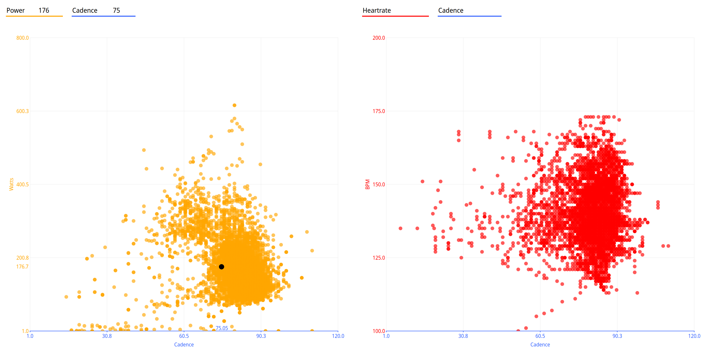
The code:
## Retrieve power and cadence
xx = GC.series(GC.SERIES_CAD)


## using qt charts
GC.setChart(title="",
            type=GC.CHART_SCATTER,
            orientation=GC_HORIZONTAL,
            legpos=GC_ALIGN_TOP,
            stack=True,
            animate=False);

yy = GC.series(GC.SERIES_WATTS)
GC.addCurve(name="Power",x=xx,y=yy,
            size=15, color="orange",
            line=0, opacity=65, opengl=False,
            xaxis="Cadence", yaxis="Watts")


yy = GC.series(GC.SERIES_HR)
GC.addCurve(name="Heartrate",x=xx,y=yy,
            size=15, color="red",
            line=0,opacity=65, opengl=False,
            xaxis="Cadence", yaxis="BPM")

GC.setAxis("Watts",min=1,max=800)
GC.setAxis("Cadence", min=1, max=120)
GC.setAxis("BPM",min=100,max=200)
GC.setAxis("Cad", min=1, max=160)
BACK: Special Topics: Overview
BACK: Table of contents