Estimating Variance Components - G-String-Legacy/GS_MV GitHub Wiki

Most of G_String's 'heavy lifting' is done in step 9 by a C++ routine called urGenova designed by Prof. Robert L. Brennan, who has kindly given his permission to include it in this software. From the raw score data, and the full set of design parameters urGenova extracts estimates of the so called 'Variance Components' for each facet and their combinations. The variance components, in turn, are then used to calculate the G-Coefficients and perform D-Analysis.

The concept of variance components stems from a mathematical theory called 'General Linear Model'. The model is called 'linear', because the the result is equal to the simple sum of a mean and various effects that determine the outcome. Although its general form is simple to write as a mathematical formula, it is somewhat obscure for non-mathematicians to understand. Instead we will first apply the concept to the example of a simple multiple choice exam, and then chat loosely about its extension to more complex cases. Fine details are not that important, and G_String knows how to do it.

So, let's start with the 58 students answering 30 MCQ questions either correctly (score 1), or incorrectly (score 0). Thus, each student can potentially get a minimum total score of 0, and a maximum of 30. The data file will have 58 rows and 31 columns. The first column contains the corresponding student index (to be ignored), the subsequent fields the individual question scores (0 or 1). The mean score over all the students and questions is 0.58966 = μ₀, which also corresponds to the probability of an average student getting the answer to an average question right.

But 'average' student, and 'average' question are theoretical constructs. In reality, students (s) differ by their ability, questions (q) by their easiness, and different students have different predilections for different kinds of questions. In generalizability jargon these deviations from average are called 'effects'.

In fact, there is a set of effects (ν) associated with each facet, as well as with their various permitted combinations. The size of each set is determined by the sample size of its facet. Thus, the General Linear Model postulates that the score (X_i,j) for student i answering question j can be expressed as:

$$ \huge X_{i,j} = \mu_0 + \nu^s_i + \nu^q_j + \nu^{sq}_{i,j} \qquad \text{(Equation 1)}$$

Where $\nu^s_i$ stands for the ability effect of student i, $\nu^q_j$ for the easiness effect of question j, and $\nu^{sq}_{i,j}$ for their cross-effect (interaction), with

$\qquad \large\sum\limits_{i=0}^{57} \nu^s_i=0 \quad {(1a)}$, $\qquad \large\sum\limits_{j=0}^{29} \nu^q_j=0 \quad {(1b)}$, and $\qquad \large\sum\limits_{i=0}^{57}\sum\limits_{j=0}^{29}\nu^{sq}_{i,j}=0 \quad {(1c)}$

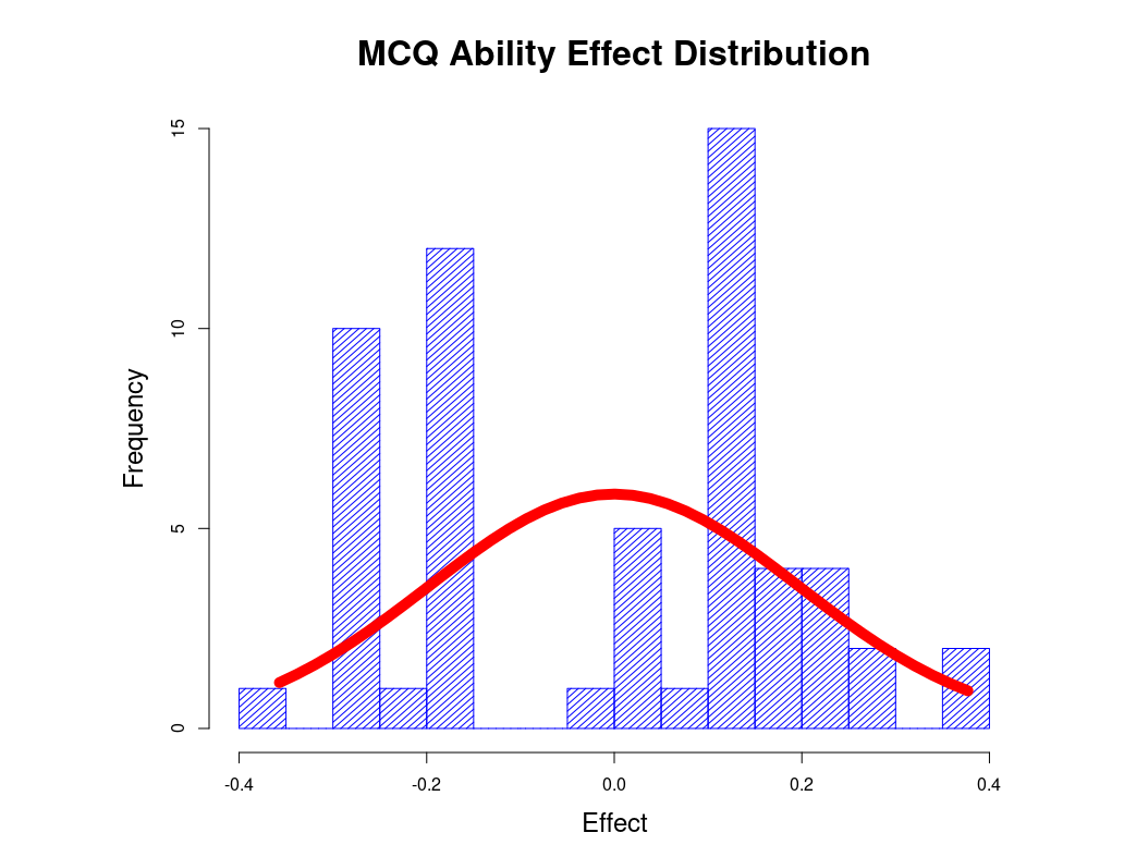
Let us now examine the properties of effects for a given facet, or interaction of facets. Since students don't know much about the ability of their colleagues, the ability effects must be considered to be random values, and because of equation (2) they must be more or less symmetrically distributed around zero, which holds for effect sets of all facets and of their interactions. As in most distributions, values get rarer, the further you move from zero. That, in fact, defines a bell-curve distribution. Each effect set distribution has its own variance, and we call these the 'variance component' of the corresponding facet. Most importantly, under the General Linear Model the variance of a sum is the sum of its component variances.

The variance components $\sigma^2_s$, $\sigma^2_q$, and $\sigma^2_{sq}$ are measures of the different effects' spread.

On this diagram the distribution of the 58 students' ability effects, as extracted by urGenova from the data file, are shown as a histogram in blue. The histogram resembles a bactrian more than a dromedary. One might be tempted to infer that the class is split into strivers and slackers. But that would be a wrong conclusion. For the data were, in fact, created by a random number generator (G_String Simulation). The variance component for students' ability comes out as $\sigma^2_s\cong 0.04$, which corresponds to a standard deviation of 0.2. The red curve shows the corresponding ideal Gaussian bell curve with a variance of 0.04. There are two reasons for the discrepancy between actual and expected data. Firstly, 58 students represent a relatively small statistical sample, and secondly, the continuous effect values can only express themselves as either score 0, or score 1, which leads to large rounding errors.

Next