Color Chart in R - EarlGlynn/colorchart GitHub Wiki
Purpose
 R is such a graphics rich tool, but the textual documentation of R's
 colors() vector, hinders an end user from quickly finding colors of interest. The Chart of R Colors in PDF format can be displayed on the screen or printed to help locate colors. Such a comparison will show colors that are reproduced reasonably well on both a display monitor and a particular printer.
In addition to simply displaying the various colors in R, this TechNote provides some details of how to work with color in R.
Background
- Why Should Engineers and Scientists Be Worried About Color?, IBM Thomas J. Watson Research Center
- Color Schemes Appropriate for Scientific Data Graphics, University of Oregon
- Package ‘RColorBrewer’
- Using RColorBrewer to colour your figures in R, R-Bloggers
- HTML Color Names
- efg's Color Reference Library, including Color: General Color Information (e.g., "color blindness", "color names", "vision"), Color Science/Theory (e.g., "color charts" and "gamuts"), Color and Computers (e.g., "calibration", "false colors", "web colors").
On many UNIX systems there is a list of color names in locations like /usr/lib/X11/rgb.txt or /etc/X11.
head /usr/lib/X11/rgb.txt
 ! $Xorg: rgb.txt,v 1.3 2000/08/17 19:54:00 cpqbld Exp $
 255 250 250 snow
 248 248 255 ghost white
 248 248 255 GhostWhite
 245 245 245 white smoke
 245 245 245 WhiteSmoke
 220 220 220 gainsboro
 255 250 240 floral white
 255 250 240 FloralWhite
 253 245 230 old lace
 . . .
For R under Windows, there is a similar rgb.txt file in allocation like C:\Program Files\R\R-3.0.2\etc\rgb.txt
Step-by-Step Procedure to learn about colors:
1. The function call, colors(), or with the British spelling, colours(), returns a vector of 657 color names in R. The color names are in alphabetical order, except for colors()[1], which is "white". The names "gray" and "grey" can be spelled either way -- many shades of grey/gray are provided with both spellings.
2. Particular color names of interest can be found if their positions in the vector are known, e.g.,
>colors()[c(552,254,26)]
[1] "red" "green" "blue"
3. grep can be used to find color names of interest, e.g.,
>grep("red",colors())
[1] 100 372 373 374 375 376 476 503 504 505 506 507 524 525 526 527 528 552 553
[20] 554 555 556 641 642 643 644 645

>colors()[grep("red",colors())]
[1] "darkred" "indianred" "indianred1" "indianred2"
[5] "indianred3" "indianred4" "mediumvioletred" "orangered"
[9] "orangered1" "orangered2" "orangered3" "orangered4"
[13] "palevioletred" "palevioletred1" "palevioletred2" "palevioletred3"
[17] "palevioletred4" "red" "red1" "red2"
[21] "red3" "red4" "violetred" "violetred1"
[25] "violetred2" "violetred3" "violetred4"

>colors()[grep("sky",colors())]
[1] "deepskyblue" "deepskyblue1" "deepskyblue2" "deepskyblue3"
[5] "deepskyblue4" "lightskyblue" "lightskyblue1" "lightskyblue2"
[9] "lightskyblue3" "lightskyblue4" "skyblue" "skyblue1"
[13] "skyblue2" "skyblue3" "skyblue4"
4. The function col2rgb can be used to extract the RGB (red-green-blue) components of a color, e.g.,
>col2rgb("yellow")
[,1]
red 255
green 255
blue 0
Each of the three RGB color components ranges from 0 to 255, which is interpreted to be 0.0 to 1.0 in RGB colorspace. With each of the RGB components having 256 possible discrete values, this results in 256256256 possible colors, or 16,777,216 colors.
While the RGB component values range from 0 to 255 in decimal, they range from hex 00 to hex FF. Black, which is RGB = (0,0,0) can be represented in hex as #000000, and white, which is RGB = (255,255,255), can represented in hex as #FFFFFF.
5. R provides a way to define an RGB triple with each of the color components ranging from 0.0 to 1.0 using the rgb function. For example, yellow can be defined:
>rgb(1.0, 1.0, 0.0)
[1] "#FFFF00"
The output is in hexadecimal ranging from 00 to FF (i.e., decimal 0 to 255) for each color component. The 0.0 to 1.0 inputs are a bit odd, but are standard in RGB color theory. Since decimal values from 0 to 255 are common, the rgb function allows a maxColorValue parameter as an alternative:
>rgb(255, 255, 0, maxColorValue=255)
[1] "#FFFF00"
The R function, GetColorHexAndDecimal, was written to display both hex and decimal values of the color components for a given color name:
GetColorHexAndDecimal <- function(color)
{
  clr <- col2rgb(color)
  sprintf("#%02X%02X%02X %3d %3d %3d", clr[1],clr[2],clr[3], clr[1], clr[2], clr[3])
}
Example:
>GetColorHexAndDecimal("yellow")
[1] "#FFFF00 255 255 0"
This GetColorHexAndDecimal function will be used below in Step 9.
6. Text of a certain color when viewed against certain backgrounds can be very hard to see, e.g., never use yellow text on a white background since there isn't good contrast between the two. One simple hueristic in defining a text color for a given background color is to pick the one that is "farthest" away from "black" or "white". One way to do this is to compute the color intensity, defined as the mean of the RGB triple, and pick "black" (intensity 0) for text color if the background intensity is greater than 127, or "white" (intensity 255) when the background intensity is less than or equal to 127.
The R function below, SetTextContrastColor, gives a good text color for a given background color name:
SetTextContrastColor <- function(color)
{
  ifelse( mean(col2rgb(color)) > 127, "black", "white")
}

# Define this array of text contrast colors that corresponds to each
# member of the colors() array.
TextContrastColor <- unlist( lapply(colors(), SetTextContrastColor) )
Examples:
>SetTextContrastColor("white")
[1] "black"
>SetTextContrastColor("black")
[1] "white"
>SetTextContrastColor("red")
[1] "white"
>SetTextContrastColor("yellow")
[1] "black"
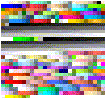
7. The following R code produces the "R Colors" graphic shown above (using SetTextContrastColor defined above):
# 1a. Plot matrix of R colors, in index order, 25 per row.
# This example plots each row of rectangles one at a time.
colCount <- 25 # number per row
rowCount <- 27

plot( c(1,colCount), c(0,rowCount), type="n", ylab="", xlab="",
  axes=FALSE, ylim=c(rowCount,0))
title("R colors")

for (j in 0:(rowCount-1))
{
  base <- j*colCount
  remaining <- length(colors()) - base
  RowSize <- ifelse(remaining < colCount, remaining, colCount)
  rect((1:RowSize)-0.5,j-0.5, (1:RowSize)+0.5,j+0.5,
    border="black",
    col=colors()[base + (1:RowSize)])
  text((1:RowSize), j, paste(base + (1:RowSize)), cex=0.7,
    col=TextContrastColor[base + (1:RowSize)])
}
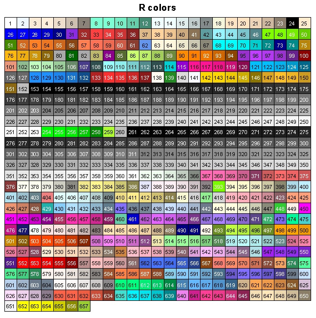
8. Alphabetical order is not necessarily a good way to find similar colors. The RGB values of each of the colors() were converted to hue-saturation-value (HSV) and then sorted by HSV. This approach groups colors of the same "hue" together a bit better. Here's the code and graphic produced:
# 1b. Plot matrix of R colors, in "hue" order, 25 per row.
# This example plots each rectangle one at a time.
RGBColors <- col2rgb(colors()[1:length(colors())])
HSVColors <- rgb2hsv( RGBColors[1,], RGBColors[2,], RGBColors[3,],
             maxColorValue=255)
HueOrder <- order( HSVColors[1,], HSVColors[2,], HSVColors[3,] )

plot(0, type="n", ylab="", xlab="",
axes=FALSE, ylim=c(rowCount,0), xlim=c(1,colCount))

title("R colors -- Sorted by Hue, Saturation, Value")

for (j in 0:(rowCount-1))
{
  for (i in 1:colCount)
  {
    k <- j*colCount + i
    if (k <= length(colors()))
    {
      rect(i-0.5,j-0.5, i+0.5,j+0.5, border="black", col=colors()[ HueOrder[k] ])
      text(i,j, paste(HueOrder[k]), cex=0.7, col=TextContrastColor[ HueOrder[k] ])
    }
  }
}
9. While the color matrices above are useful, a more useful display would include a rectangular area showing the color, the color index, the color name, and the RGB values, both in hexadecimal, which is often used on web pages.
The code for this is a bit tedious -- see Item #2 in the ColorChart.R code for complete details.
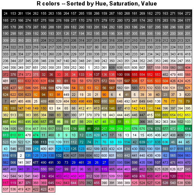
Here is the first page of the Chart of R colors:
10. R Code to create Color Chart (named ColorChart.pdf) with all the graphics shown on this page.