Here you can find some example code which produces automatic figures from a model, in the below example, the code will produce a unified figure for each predictor, showing a triplanar view:

Here, we assume you have a dataframe data which contains all your information.

library(grid)
library(tidyverse)
library(MRIcrotome)
library(RMINC)
library(magrittr) #to be able to use "%>%"

## HERE GOES CODE TO SETUP DATAFRAME ETC ##

anatVol <- mincArray(mincGetVolume("template.mnc"))
averagemask <- mincArray(mincGetVolume("ask.mnc"))

model = mincLmer(relative ~ poly(age,2)*sex + (1|subject) + (1|dataset), data = data, mask = "mask.mnc", parallel = c("local",20))
model = mincLmerEstimateDF(model)
thresholds = attr(mincFDR(model), "thresholds")
print(thresholds)

#Here we figure out the extent of the mask, so we can use it to limit
# the FOV
# You may want to adjust these slighty buy adding/subtracting, so you don't
# quite go to the edge of the mask
dim1_begin <- min(which(averagemask == 1, arr.ind=TRUE)[,"dim1"])
dim1_end <-max(which(averagemask == 1, arr.ind=TRUE)[,"dim1"])
dim2_begin <- min(which(averagemask == 1, arr.ind=TRUE)[,"dim2"])
dim2_end <- max(which(averagemask == 1, arr.ind=TRUE)[,"dim2"])
dim3_begin <- min(which(averagemask == 1, arr.ind=TRUE)[,"dim3"])
dim3_end <- max(which(averagemask == 1, arr.ind=TRUE)[,"dim3"])

jacobian="relative"

# If your model is instead a mincLm, you need to use this loop command
# #for (predictor in dimnames(thresholds)[2](/CoBrALab/documentation/wiki/2)[c(-1,-2)]) {

for (predictor in dimnames(thresholds)[2](/CoBrALab/documentation/wiki/2)[c(-1)]) {
 
  #If you want to save this to a file, uncomment next line
  #svg(paste0("results/human_",jacobian,"_",predictor,".svg"), height = 3.1, width = 4)
  #We use a tryCatch here to keep going if there's some kind of error in a an individual plot
  tryCatch({
  #Here, we extract the thresholds from the code, and clip them to 2 digits, otherwise the plotting doesn't look good
  lowerthreshold = round(thresholds["0.05",predictor],digits=2)
  #Sometimes, there isn't an 0.01 threshold, when thats the case, we use the max instead, be careful to read the threshold array printed above
  upperthreshold = round(ifelse(is.na(thresholds["0.01",predictor]), max(c(max(mincArray(model, predictor)),abs(min(mincArray(model, predictor))))), thresholds["0.01",predictor]),digits=2)
  # Here is the plotting code, we do all three slice directions in one figure. This was optimized for a human brain, you may need to
  # adjust the nrow and ncol to get exactly the figure you want
  # You will also need to adjust the anatVol low and high values to correspond to good thresholds for your template
  sliceSeries(nrow = 5, ncol = 2, dimension = 2, begin = dim2_begin, end = dim2_end) %>%  
    anatomy(anatVol, low=1, high=5.9) %>%
    addtitle("Coronal") %>%
    overlay(mincArray(model, predictor),
      low=lowerthreshold, 
      high=upperthreshold, 
      symmetric = T, alpha=0.6) %>%
    sliceSeries(nrow = 6, ncol= 2, dimension = 1, begin = dim1_begin, end = dim1_end) %>%  
    anatomy(anatVol, low=1, high=5.9) %>%
    addtitle("Sagittal") %>%
    overlay(mincArray(model, predictor),   
      low=lowerthreshold,
      high=upperthreshold,
      symmetric = T, alpha=0.6) %>%
    sliceSeries(nrow = 5, ncol= 2, dimension = 3, begin = dim3_begin, end = dim3_end) %>% 
    anatomy(anatVol, low=1, high=5.9) %>%
    addtitle("Axial") %>%
    overlay(mincArray(model, predictor),
      low=lowerthreshold,
      high=upperthreshold,
      symmetric = T, alpha=0.6) %>%
    legend(predictor) %>%
    draw()}, error=function(e){cat("ERROR :",conditionMessage(e), "\n")})
  #If you are saving to file, also uncomment this
  #dev.off()
}

Multiple figures

Here, we adjust the code to generate three figures, one for each view:

jacobian="relative"

for (predictor in dimnames(thresholds)[2](/CoBrALab/documentation/wiki/2)[-1]) {

  #We use a tryCatch here to keep going if there's some kind of error in a an individual plot
  tryCatch({
  #Here, we extract the thresholds from the code, and clip them to 2 digits, otherwise the plotting doesn't look good
  lowerthreshold = round(thresholds["0.05",predictor],digits=2)
  #Sometimes, there isn't an 0.01 threshold, when thats the case, we use the max instead, be careful to read the threshold array printed above
  upperthreshold = round(ifelse(is.na(thresholds["0.01",predictor]), max(c(max(mincArray(model, predictor)),abs(min(mincArray(model, predictor))))), thresholds["0.01",predictor]),digits=2)
  #svg(paste0("results/",jacobian,"_",predictor,"_coronal.svg"), height = 3.1, width = 4)
  sliceSeries(nrow = 5, ncol= 6, begin = dim2_begin, end = dim2_end, dimension = 2) %>%  #slice sequence to display stats
    anatomy(anatVol, low=1, high=5.9) %>%
    overlay(mincArray(model, predictor),     # specify which column of the mincLM model
            low=lowerthreshold, high=upperthreshold, symmetric = T, alpha=0.6) %>%       # t score range; symmetric = T means show positive and negative t values
    legend(predictor) %>%
    contourSliceIndicator(anatVol, c(1.8, 2), slice=125) %>%
    draw()
  #dev.off()

  #svg(paste0("results/",jacobian,"_",predictor,"_sagittal.svg"), height = 3.1, width = 4)
  sliceSeries(nrow = 5, ncol= 5, begin = dim1_begin, end = dim1_end, dimension = 1) %>%  #slice sequence to display stats
    anatomy(anatVol, low=1, high=5.9) %>%
    overlay(mincArray(model, predictor),     # specify which column of the mincLM model
            low=lowerthreshold, high=upperthreshold, symmetric = T, alpha=0.6) %>%       # t score range; symmetric = T means show positive and negative t values
    contourSliceIndicator(anatVol, c(1.8, 2), slice=125) %>%
    legend(predictor) %>%
    draw()
  #dev.off()

  #svg(paste0("results/",jacobian,"_",predictor,"_axial.svg"), height = 3.1, width = 4)
  sliceSeries(nrow = 4, ncol= 6, begin = dim3_begin, end = dim3_end, dimension = 3) %>%  #slice sequence to display stats
    anatomy(anatVol, low=1, high=5.9) %>%
    overlay(mincArray(model, predictor),     # specify which column of the mincLM model
            low=lowerthreshold, high=upperthreshold, symmetric = T, alpha=0.6) %>%       # t score range; symmetric = T means show positive and negative t values
    legend(predictor) %>%
    contourSliceIndicator(anatVol, c(1.8, 2), slice=125) %>%
    draw()
  #dev.off()
     }, error=function(e){cat("ERROR :",conditionMessage(e), "\n")})
}

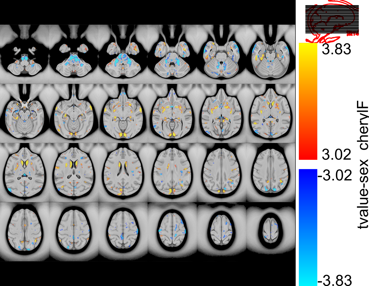
Automatic Visualization with transparent thresholds

library(grid)
library(tidyverse)
library(MRIcrotome)
library(RMINC)
library(magrittr) #to be able to use "%>%"

## HERE GOES CODE TO SETUP DATAFRAME ETC ##

anatVol <- mincArray(mincGetVolume("template.mnc"))
averagemask <- mincArray(mincGetVolume("ask.mnc"))

model = mincLmer(relative ~ poly(age,2)*sex + (1|subject) + (1|dataset), data = data, mask = "mask.mnc", parallel = c("local",20))
model = mincLmerEstimateDF(model)
thresholds = attr(mincFDR(model), "thresholds")
print(thresholds)

#Here we figure out the extent of the mask, so we can use it to limit
# the FOV
# You may want to adjust these slighty buy adding/subtracting, so you don't
# quite go to the edge of the mask
dim1_begin <- min(which(averagemask == 1, arr.ind=TRUE)[,"dim1"])
dim1_end <-max(which(averagemask == 1, arr.ind=TRUE)[,"dim1"])
dim2_begin <- min(which(averagemask == 1, arr.ind=TRUE)[,"dim2"])
dim2_end <- max(which(averagemask == 1, arr.ind=TRUE)[,"dim2"])
dim3_begin <- min(which(averagemask == 1, arr.ind=TRUE)[,"dim3"])
dim3_end <- max(which(averagemask == 1, arr.ind=TRUE)[,"dim3"])

jacobian="relative"

# If your model is instead a mincLm, you need to use this loop command
# #for (predictor in dimnames(thresholds)[2](/CoBrALab/documentation/wiki/2)[c(-1,-2)]) {

for (predictor in dimnames(thresholds)[2](/CoBrALab/documentation/wiki/2)[c(-1)]) {
 
  #If you want to save this to a file, uncomment next line
  #svg(paste0("results/human_",jacobian,"_",predictor,".svg"), height = 3.1, width = 4)
  #We use a tryCatch here to keep going if there's some kind of error in a an individual plot
  tryCatch({
  #Here, we extract the thresholds from the code, and clip them to 2 digits, otherwise the plotting doesn't look good
  lowerthreshold = round(thresholds["0.05",predictor],digits=2)
  #Sometimes, there isn't an 0.01 threshold, when thats the case, we use the max instead, be careful to read the threshold array printed above
  upperthreshold = round(ifelse(is.na(thresholds["0.01",predictor]), max(c(max(mincArray(model, predictor)),abs(min(mincArray(model, predictor))))), thresholds["0.01",predictor]),digits=2)

# Generate the default colourmaps
pospal = colorRampPalette(c("red", "yellow"), alpha=TRUE)(255)
negpal = colorRampPalette(c("blue", "turquoise1"), alpha=TRUE)(255)

  # Find the crossover point in the map where the colourmap switches to "non transparent"
  # Need to include the alpha term here, but its always opaque
  breakpointpos = pospal[round(lowerthreshold/upperthreshold*255) - 1]
  breakpointneg = negpal[round(lowerthreshold/upperthreshold*255) - 1]

  # Generate a subset of the colourmap now which ramps from the same starting point and ends at breakpoint, with full opacity
  pospalalpha = colorRampPalette(c("#FF000000", breakpointpos), alpha=TRUE)(round(lowerthreshold/upperthreshold*255) - 1)
  negpalalpha = colorRampPalette(c("#0000FF00", breakpointneg), alpha=TRUE)(round(lowerthreshold/upperthreshold*255) - 1)

  # Concatenate the two maps together for a complete map
  combinedpospal = c(pospalalpha, pospal[round(lowerthreshold/upperthreshold*255):length(pospal)])
  combinednegpal = c(negpalalpha, negpal[round(lowerthreshold/upperthreshold*255):length(negpal)])


  # Here is the plotting code, we do all three slice directions in one figure. This was optimized for a human brain, you may need to
  # adjust the nrow and ncol to get exactly the figure you want
  # You will also need to adjust the anatVol low and high values to correspond to good thresholds for your template
  sliceSeries(nrow = 5, ncol = 2, dimension = 2, begin = dim2_begin, end = dim2_end) %>%  
    anatomy(anatVol, low=1, high=5.9) %>%
    addtitle("Coronal") %>%
    overlay(mincArray(model, predictor),
          low = 0,
          high = upperthreshold,
          col = combinedpospal,
          rCol = combinednegpal,
      symmetric = T) %>%
    contours(abs(mincArray(model, predictor)), levels=lowerthreshold, lwd=2, col="black") %>%
    sliceSeries(nrow = 6, ncol= 2, dimension = 1, begin = dim1_begin, end = dim1_end) %>%  
    anatomy(anatVol, low=1, high=5.9) %>%
    addtitle("Sagittal") %>%
    overlay(mincArray(model, predictor),   
          low = 0,
          high = upperthreshold,
          col = combinedpospal,
          rCol = combinednegpal,
      symmetric = T) %>%
  contours(abs(mincArray(model, predictor)), levels=lowerthreshold, lwd=2, col="black") %>%    
  sliceSeries(nrow = 5, ncol= 2, dimension = 3, begin = dim3_begin, end = dim3_end) %>% 
    anatomy(anatVol, low=1, high=5.9) %>%
    addtitle("Axial") %>%
    overlay(mincArray(model, predictor),
          low = 0,
          high = upperthreshold,
          col = combinedpospal,
          rCol = combinednegpal,
      symmetric = T) %>%
    legend(predictor) %>%
  contours(abs(mincArray(model, predictor)), levels=lowerthreshold, lwd=2, col="black") %>%
    draw()}, error=function(e){cat("ERROR :",conditionMessage(e), "\n")})
  #If you are saving to file, also uncomment this
  #dev.off()