[PAN sharpening 2]DSen2 - ChaeyeonSon/PaperReading GitHub Wiki
Super resolution of Sentinel 2 images: Learning a globally applicable deep neural network
https://arxiv.org/pdf/1803.04271.pdf
- Sentinel-2 위성영상은 13개의 spectral band로 되어있고, virtually infinite 한 양의 데이터로 매우 다양한 기후와 지형을 커버하고 있다.
- 학습은 real Sentinel-2를 downsampling 한 LR에서 학습하여 40->20m GSD, 360->60m GSD 학습.
- RMSE에서는 기존보다 거의 50퍼정도 좋은 성능을 보이고, spectral 특징 보존을 더욱 잘한다.
1. Introduction
- 각 spectrum band는 viewing direction이 같지만 storage&transmission BW제한으로 Resolution이 2-6(20m, 60m GSD)으로 각각 다르다.
- 목표는 모든 band가 가장 높은 spatial resolution(10m GSD)에서 사용할 수 있게 하는 것이다.
- S2는 공짜로 world-wide coverage한 데이터를 사용할 수 있어 중요하기에 특별히 이 데이터에 대해 SR 진행.
- 기존의 naive 방식은 blurry하거나 additional information이 거의 없어 CNN 같은 smart한 upsampling 방식 적용.
- 목표는 기존 밴드의 spectral information를 보존하면서 최고의 reconstruction 정확도
- 2개의 CNN(20m->10m GSD : 40m->20m 로 학습 ; 60m -> 10m GSD : 360m->60m로 학습; => 합성적으로 downsample org S2 img)
- 합성 데이터에서 실험 결과-> mapping 은 large extent scale-invariant하며 reduced resolution에서 학습가능하다는 주장 지지.
- single model(S2)에 대해 학습했음에도 S2 data의 광범위함 덕분에 특정 context에 overfit되지 않고 성능도 기존보다도 뛰어남.
특징 : 1. 높은 정확도의 모든 super-resolved band, 2. 더 좋은 spectral 특성 보존, 3. 좋아진 연산 속도, 4. retraining 없어도 S2만으로 글로벌한 적용, 5. end-2-end system, retrain도 가능, 6. free, publicly 이용가능한 코드와 네트워크 weight
2. Related Work
3. Input data
Sentinel 2A, 2B
남극 빼고 모든 지형 커버, 13 band의 multispectral images
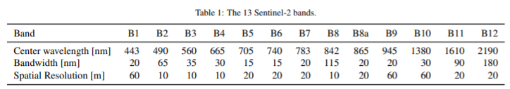
- 10m와 20m : general land-cover mapping, 농경, 숲 등...
- 3개의 60m : water vapour, aerosol corrections, cirrus clouds estimation
- 첫 10개는 VNIR spectrum, 마지막 3개는 SWIR spectrum
- Clerc and MPC Team(2018)에 의하면 S2는 band끼리 잘못 등록된 것도 거의 없어 높은 confidence를 갖는 데이터 셋이다.(?)
- B10 제외
- Copernicus Services Data Hub에서 무료 다운 가능
- 이 실험에서 2A(12.2016~ 11.2017), 2B(07.2017~ 11.2017)를 사용하였으며 global 하게 적용되도록 기후, 지형따라 다양하게 randomly 뽑히게하였고, undefined pixel이 있는 tile은 사용하지 않는다.
4. Method
4.1. Simulation process
hr에서 lr로 spatial detail의 transfer는 scale-invariant 하므로 relative resolution 차이에만 의존한다. relations between bands of different resolutions are self-similar within the relevant scale range??
약한 self-similarity만 필요하므로 굳이 'blind' generative mapping은 필요 없다.
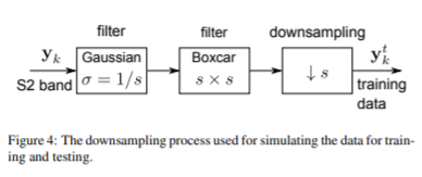
scale invariance : 20m->10m는 40m>20m 로 downsampling 해서 학습; 10m 20m 60m 도 학습은 60m 120m 360m 로.
10m super-resolved band는 visual로만 체크.
4.2. 20m and 60m resolution network
A={B2, B3, B4, B8}(GSD=10), B={B5, B6, B7, B8A, B11, B12}(GSD=20), C={B1, B9}(GSD=60)
두개의 네트워크 순서대로 20m->10m; 60m->10m
4.3. Basic architecture
EDSR이 기본 구조로 사용
lambda=0.1
BN이 없는 이유는 이미지의 flexibility를 줄이는 역할을 하기 때문이다.
skip connection -> complete network learns the additive correction from the bilinearly upsampled image to the desired ouput.??
4.4. Deep and very deep networks
- d= 6, f=128 : 14 conv, 1.8M weights (DSen)
- d= 32, f=256 : 66 conv, 37.8M weights (VDSen)
very deep이 학습 시간은 2배, 예측 시간은 5배까지 느리며 free parameter 증가 대비 gain 이 적다.
4.5. Training details
- 수렴이 빠르고 결과가 잘 전달되므로 L1 사용
- small random values with HeUniform method로 initialize.
- Adam variant of SGD, Nesterov momentum
- 32x32 for T, 96x96 for S patch로 학습 => low-level의 local texture와 small semantic structures(buildings, small waterbodies ...) 를 잡을 수 있다.
- We do not expect the latter to hold much information about the local pixel values, instead there is a certain danger that the large-scale layout of a limited training set it is too unique to generalise to unseen locations.??
- 예측 단계의 타일크기는 GPU 메모리에 의해 정해지며 boundary artifact를 피하고자 인접 타일들은 cropped with an overlap of 2 low-resolution input pixels, corresponding to 40 m for T2×, respectively 120 m for S6×. ??
5. Experimental Results
5.1. Implementation details
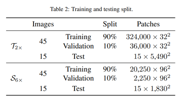
15 test images, each with a size of 110×110 km^2 -> 5490×5490 pixels at 20 m GSD /1830×1830 pixels at 60 m GSD.
lr = 1e-4 -> 5 연속 epoch만큼 validation loss가 감소하지 않으면 0.5만큼 감소
5.2. Baselines and evaluation metrics
SRE : signal to reconstruction error ratio : measures the error relative to the power of the signal
SAM : spectral angle mapper : the angular deviation between true and estimated spectral signatures, complimentary to the
two previous ones, and quite useful for some applications, in that it measures how faithful the relative spectral distribution of a pixel is reconstructed, while ignoring absolute brightness.
UIQ : universal image quality index : evaluates the reconstructed image in terms of luminance, contrast, and structure
5.3. Evaluation at lower scale
- 2x upsampling(40m->20m)
Superres 같은 최신 기술보다 RMSE를 48% 감소 외에도 모두 우세, VDSen이 DSen보다 전체적으로 성능이 더 뛰어나긴 하다.
80m->40m 실험도 진행; 40->20보다는 결과가 나쁘지만 다른 baseline들보다는 우세 => lower scale training이 합리적이다.
- 6x upsampling(360m->60m)
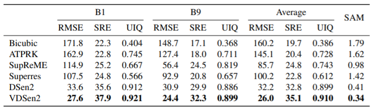
upsampling 배율이 높을수록 VDSen이 DSen보다 더 성능이 좋다.
2x upsampling보다 baselines 대비 성능 향상이 더욱 좋다.
5.4. Evaluation at the original scale
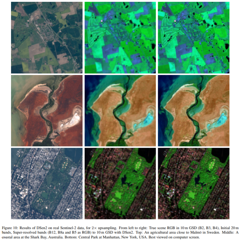
ground truth가 없으므로 육안 검사를 하는데 눈으로 보기에는 결과들이 10m GSD 품질의 이미지들과 perceptual quality가 비슷해 보인다.
5.5. Suitability of pan-sharpening methods
best-performing PAN sharpening methods
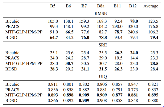
Pan-Sharpening은 검증된 SR을 대신할 수 없으며, Sentinel-2에 적합하지 않다.
많은 논문들이 대역별 오류를 보여주지 않아서 B11과 B12에서 어려움이 가려진다.
그런데 본인은 PAN으로 4 channel 사용해놓고 비교 모델들은 1 channel 사용... 사기다...
6. Discussion
6.1. Different network configurations
- DSen2같은 적당한 크기의 네트워크는 충분히 좋은 성능을 보인다.
- VDSen2같은 매우 깊은 네트워크는 gain의 효율이 좋지 않고, 특이하게 오버핏 경향이 강하지 않다.
- 모래시계처럼 생긴 구조 지양, pooling은 local detail을 떨어뜨릴 위험이 있기 때문.
- 적절한 depth? 하드웨어만 준비되어 있다면 VDSen이 DSen보다 나을 수도... 하지만 GPU 제한되어있다면 DSen이 좋다.
- 상대적으로 쉬운 지상의 커버나 정확도가 크게 필요하지 않다면 DSen(d=6)보다도 block 개수 낮출 수도 있다.
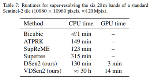
6.2 Timing